SiO2 crystal (Gamma-point) with a Jastrow-Slater single-determinant ansatz via VMC and LRDMC using ECPs

00 Introduction

In this tutorial, you will perform a VMC/LRDMC workflow for crystalline SiO2 under PBCs, starting from a PySCF DFT calculation with ccECPs. You will use Gamma-point sampling. All input and output files for this tutorial can be downloaded here.

01 PySCF calculation and its conversion to a TREXIO file

The first step of this tutorial is to generate a JDFT ansatz using PySCF. Run a PySCF calculation by typing as follows. The Python script will be presented later.

cd 01_pyscf_calculation
python3 pyscf_SiO2.py

You can convert the generated PySCF checkpoint file to a TREXIO file

# pyscf chkfile to TREXIO
trexio convert-from -t pyscf -i SiO2.chk -b hdf5 SiO2.hdf5

02 From TREXIO file to TurboRVB WF

Next, we convert the TREXIO file to a TurboRVB wavefunction file. It can be done by using trexio-to-turborvb program in the TurboGenius package as follows:

trexio-to-turborvb SiO2.hdf5 -jasbasis cc-pVDZ -jascutbasis

Note

If you want to specify Jastrow basis set, you can use the following python script to convert the TREXIO file.

vi trexio_turborvb_wf_converter.py # define your Jastrow basis
python trexio_turborvb_wf_converter.py

03 JDFT ansatz - Jastrow optimization

One should refer to the Hydrogen tutorial for the details. Here, only needed commands are shown.

1. Copy the wavefunction file and the pseudopotential file:

cd ../02_optimization/
cp ../01_pyscf_calculation/fort.10 fort.10
cp ../01_pyscf_calculation/pseudo.dat .
cp fort.10 fort.10_pyscf

2. Generate an input file datasmin.input:

turbogenius vmcopt -g -opt_onebody -opt_twobody -opt_jas_mat -optimizer lr -vmcoptsteps 300 -steps 1000 -nw 1024 -learn 0.30 -reg -0.01 -maxtime 86000

3. Run the optimization:

export TURBOVMC_RUN_COMMAND="mpirun -np 16 turborvb-mpi.x"
turbogenius vmcopt -r

See Note in the optimization step for the ways to run the calculations.

4. Perform the postprocess and plot the results:

turbogenius vmcopt -post -optwarmup 80 -plot

Check plot_energy_and_devmax.png and the files in the parameters_graphs directory.

Note

Optimization tips:

• In the natural gradient method, a matrix \(S\) is regularized as \({\rm diag}(S') = (1 + {\rm parr}) {\rm diag}(S)\) before calculating \({S'}^{-1}\) for a positive value of the parr parameter (specified by the -reg option). When \(S\) is much ill-conditioned, the above regularization does not work. Instead, by choosing a negative value of the parr parameter, \({\rm diag}(S') = {\rm diag}(S) + {\rm parr}\) is adopted in which the diagonal part is directly enhanced by the parr parameter. This may stabilize the inversion.

• By adding -num_opt_param to the turbogenius command line or specifying a parameter npbra in the &optimization section of the input parameter datasmin.input, the convergence may speed up. The figure below plots the values of devmax along the optimization steps, with and without specifying npbra.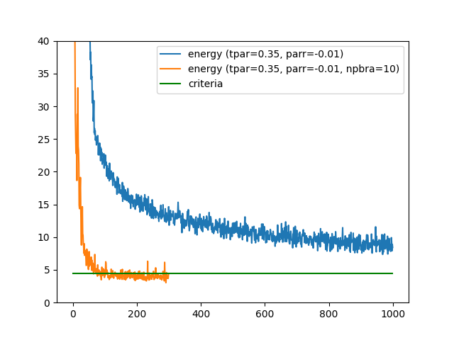

  

04 JDFT ansatz - VMC

The next step is to run a single-shot VMC calculation. This is done using the vmc module of TurboGenius. First, prepare the wavefunction and related files:

cd ../03_vmc/
cp ../02_optimization/fort.10 fort.10
cp ../02_optimization/pseudo.dat .

Next, generate an input file datasvmc.input using:

turbogenius vmc -g -steps 1000 -nw 128

Then, run the VMC calculation:

TURBOVMC_RUN_COMMAND="mpirun -np 16 turborvb-mpi.x"
export TURBOVMC_RUN_COMMAND

turbogenius vmc -r

Finally, run the postprocess:

turbogenius vmc -post -bin 10 -warmup 5

Check the reblocked total energy and error in the file pip0.d.

05 JDFT ansatz - LRDMC

Now we proceed to the lattice regularized diffusion Monte Carlo calculation that can improve a trial wavefunction obtained by a DFT calculation or a VMC optimization. One should refer to the Hydrogen tutorial for the details.

In this section, we will perform the calculation at the lattice constant alat=0.20. First, copy the prepared wavefunction and the pseudopotential files:

# LRDMC run
cd ../04_lrdmc/
cp ../03_vmc/fort.10 .
cp ../03_vmc/pseudo.dat .

Next, generate an input file datasfn.input for the LRDMC calculation:

turbogenius lrdmc -g -etry -108.00 -alat -0.20 -steps 1000 -nw 128

Then, run the calculation by typing:

TURBOVMC_RUN_COMMAND="mpirun -np 16 turborvb-mpi.x"
export TURBOVMC_RUN_COMMAND

turbogenius lrdmc -r

Finally, run the postprocess:

turbogenius lrdmc -post -bin 20 -corr 3 -warmup 5

We wil get E at a=0.20 bohr in pip0_fn.d.

One then follows the above procedure for several choices of alat, and extrapolates the energy value at \(a \to 0\). See the Hydrogen tutorial for the concrete steps.

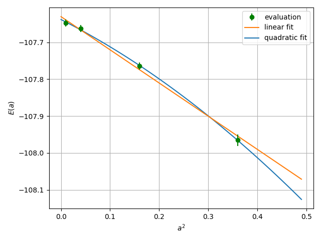
Extrapolation of the energy value at \(a \to 0\) using the linear and quadratic fits with respect to \(a^2\).