A more flexible ansatz: the hydrogen dimer with a Jastrow–Antisymmetrized Geminal Power (JAGP) ansatz via VMC and lattice-regularized DMC (LRDMC)
In this tutorial, you will compute all-electron VMC and LRDMC energies of the hydrogen dimer (\(H_2\)). You will go beyond the Jastrow–Slater single-determinant ansatz by adopting a JAGP wave function. All input and output files for this tutorial can be downloaded here.
06 Convert JDFT WF to JAGP one
We assume that we have finished all JDFT calculations following the steps described in the previous tutorial.
The next step is to convert the optimized JDFT ansatz to a JAGPs one.This can be done using convertfort10 module of Turbo-Genius. Basically, we require two fort.10 files: the JDFT one (that we want to convert) and a JAGPs fort10 file which we will use as a template for conversion. The JDFT one should be named as fort.10_in and the JAGPs one should be named as fort.10_out.
Copy fort.10 in 03_vmc to 06_convert.
cd ./06_convert/
cp ../../01Hydrogen_dimer_pyscf/03_vmc/fort.10 .
cp ../../01Hydrogen_dimer_pyscf/03_vmc/pseudo.dat .

turbogenius convertwf -to agps
Warning
the original fort.10 is renamed to fort.10_bak
Please check the overlap square in out_conv:
# grep Overlap out_conv
....
Overlap square with no zero  0.9999....
Overlap square should be close to unity, i.e., if the conversion is perfect, this becomes unity.
The conversion has finished. The obtained JAGPs wavefunction is fort.10.
07 Conversion check
We recommend you should check if the above conversion was successful. This can be checked using the so-called correlated sampling method. Indeed, one can check the difference in energies of WFs using a VMC calculation.
Copy the obtained JAGPs wavefunction fort.10, and the optimized JDFT wavefunction fort.10_in as fort.10_corr:
cd ../07_conversion_check/
cp ../06_convert/fort.10 ./fort.10
cp ../06_convert/fort.10_bak ./fort.10_corr
cp ../06_convert/pseudo.dat .
Prepare input files using:
turbogenius correlated-sampling -g -steps 100 -nw 128
For the correlating sampling, we need two input files, for a vmc calculation (i.e., generation of Markov chain) and a correlated sampling itself.
The generated datasvmc.input looks like:
&simulation
itestr4=2
ngen=100
maxtime=3600
iopt=1
disk_io='mpiio'
/
&pseudo
/
&vmc
/
&readio
iread=3
/
¶meters
/
&kpoints
/
and readforward.input looks like:
&simulation
/

&system
/

&corrfun
    bin_length=2
    initial_bin=1
    correlated_samp=.true.
/
Now run the calculation using:
export TURBOVMC_RUN_COMMAND="mpirun -np 16 turborvb-mpi.x"
export TURBOREADFORWARD_RUN_COMMAND="mpirun -np 16 readforward-mpi.x"

turbogenius correlated-sampling -r
corrsampling.dat contains the output.
# corrsampling.dat
Energy (fort10 ref.) = -1.17606202 Ha +- 0.00119647941 Ha
Energy (fort10 corr.) = -1.17606265 Ha +- 0.00119634713 Ha
Energy difference = 6.26299353e-07 Ha +- 2.29651078e-06 Ha
Overlap square = 0.999999977 +- 6.05288029e-08
reweighted difference indicates the difference in energies of the WFs, fort.10 and fort.10_corr. This should be close to zero. Overlap square should be close to unity, i.e., if a conversion is perfect, this becomes unity.
08 Nodal surface optimization (WF=JsAGPs)
In this step, the Jastrow factors and the determinant part are optimized at the VMC level using vmcopt module of Turbo-Genius. The procedure is almost the same as in 02 Jastrow factor optimization (WF=JDFT)
First of all, copy the converted wavefunction fort.10
cd ../08_nodal_surface_optimization/
cp ../06_convert/fort.10 .
cp ../06_convert/pseudo.dat .
To generate datasmin.input, which is a minimal input file for a VMC-optimization use:
turbogenius vmcopt -g -opt_onebody -opt_twobody -opt_jas_mat -opt_det_mat -optimizer lr -vmcoptsteps 1000 -steps 100 -nw 128
The input file should look something like:
&simulation
itestr4=-4
ngen=100000
iopt=1
maxtime=86400
disk_io='mpiio'
/
&pseudo
npsamax=4
/
&vmc
/
&optimization
ncg=1
nweight=100
nbinr=1
iboot=0
tpar=0.3
parr=0.0001
iesdonebodyoff=.false.
iesdtwobodyoff=.false.
twobodyoff=.false.
/
&readio
/
¶meters
iesd=1
iesfree=1
iessw=1
iesup=0
iesm=0
/
&kpoints
/
&dynamic
/
Now run VMC optimization using:
export TURBOVMC_RUN_COMMAND="mpirun -np 16 turborvb-mpi.x"
turbogenius vmcopt -r
Now for post-processing use:
turbogenius vmcopt -post -optwarmup 80 -plot
It plots energy with the error bars and devmax wrt optimization steps (plot_energy_and_devmax.png).
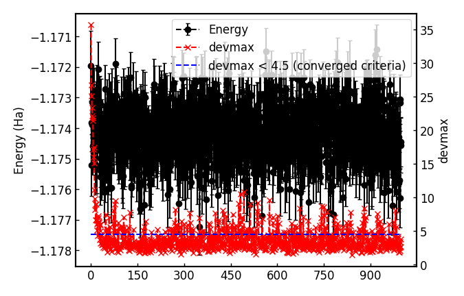
For the hydrogen dimer, the JDFT ansatz is enough accurate, so nothing has gained.
09 VMC (WF=JsAGPs)
The same as in the JDFT case. See 03 VMC (WF=JDFT)
First, copy fort.10 from 08_nodal_surface_optimization to 09_vmc.
cd ../09_vmc
cp ../08_nodal_surface_optimization/fort.10 fort.10
cp ../08_nodal_surface_optimization/pseudo.dat .
Now generate the input file for vmc datasvmc.input using:
turbogenius vmc -g -steps 1000 -nw 128
Run a VMC calculation by typing:
export TURBOVMC_RUN_COMMAND="mpirun -np 16 turborvb-mpi.x"
turbogenius vmc -r
After the VMC run finishes, use post-processing to check the total energy:
turbogenius vmc -post -bin 10 -warmup 5
# this corresponds to forcevmc.sh 10 5 1
Use the following values in this example:
bin length = 10
init bin = 5
pulay = 1 (default)

Chosen values: bin=10, init_bin=5, pulay=1, => equil_steps=50

# Note: this corresponds to ``forces_vmc.sh 10 5 1``
Postprocessing basically does reblocking using the binning technique. Here again post-processing has two modes: manual and interactive.
The reblocked total energy and error are written to the file energy_error.out.
More details are provided in the file pip0.d.
% cat pip0.d
Energy =  -1.17399712181874  4.494314925096871E-004
10 LRDMC (WF=JsAGPs)
The same as in the JDFT case. See 04 LRDMC (WF=JDFT)
cd ../10_lrdmc/
cp ../09_vmc/fort.10 .
cp ../09_vmc/pseudo.dat .

turbogenius lrdmc -g -etry -1.10 -alat -0.20 -steps 1000 -nw 128
Now run the LRDMC calculation:
export TURBOVMC_RUN_COMMAND="mpirun -np 16 turborvb-mpi.x"
turbogenius lrdmc -r
For post-processing use:
turbogenius lrdmc -post -bin 20 -corr 3 -warmup 5
# This corresponds to forcefn.sh 20 3 5 1
Thus, we get \(E (a=0.20 {\rm bohr})\) = -1.1739(4) Ha.
11 Summary
Total energy:
DFT (PZ-LDA) = -1.1373 Ha
VMC (JDFT) = -1.1727(7) Ha
VMC (JAGPs) = -1.1749(4) Ha
LRDMC (JDFT at a=0.20 bohr) = -1.1744(7) Ha.
LRDMC (JAGPs at a=0.20 bohr) = -1.1739(4) Ha.
CCSD(T)=FULL/cc-pVQZ = -1.173793 Ha (Computational Chemistry Comparison and Benchmark DataBase)