Ammonia with a Jastrow–Slater single-determinant ansatz via VMC and LRDMC using effective core potentials (ECPs)

00 Introduction 

In this tutorial, you will learn a complete workflow for VMC and LRDMC calculations on the ammonia molecule, starting from a DFT calculation in PySCF that employs correlation-consistent effective core potentials (ccECPs). All input and output files for this tutorial can be downloaded here.

01 PySCF calculation and its conversion to a TREXIO file 

The first step is to run a PySCF calculation by typing:

# pyscf calculation
cd 01_pyscf_calculation
python3 pyscf_NH3.py

The Python code is given as follows:

#!/usr/bin/env python
# coding: utf-8

# pySCF -> pyscf checkpoint file (NH3 molecule)

# load python packages
import os, sys

# load ASE modules
from ase.io import read

# load pyscf packages
from pyscf import gto, scf, mp, tools
 
#open boundary condition
structure_file="NH3.xyz"
checkpoint_file="NH3.chk"
pyscf_output="out_NH3_pyscf"
charge=0
spin=0
basis="ccecp-ccpvtz"
ecp='ccecp'
scf_method="HF"  # HF or DFT
dft_xc="LDA_X,LDA_C_PZ" # XC for DFT

print(f"structure file = {structure_file}")

# read a structure
atom=read(structure_file)
chemical_symbols=atom.get_chemical_symbols()
positions=atom.get_positions()
mol_string=""
for chemical_symbol, position in zip(chemical_symbols, positions):
    mol_string+="{:s} {:.10f} {:.10f} {:.10f} \n".format(chemical_symbol, position[0], position[1], position[2])

# build a molecule
mol = gto.Mole()
mol.atom = mol_string
mol.verbose = 5
mol.output = pyscf_output
mol.unit = 'A' # angstrom
mol.charge = charge
mol.spin = spin
mol.symmetry = False

# basis set
mol.basis = basis

# define ecp
mol.ecp = ecp

# molecular build
mol.build(cart=False)  # cart = False => use spherical basis!!

# calc type setting
print(f"scf_method = {scf_method}")  # HF/DFT

if scf_method == "HF":
    # HF calculation
    if mol.spin == 0:
        print("HF kernel = RHF")
        mf = scf.RHF(mol)
        mf.chkfile = checkpoint_file
    else:
        print("HF kernel = ROHF")
        mf = scf.ROHF(mol)
        mf.chkfile = checkpoint_file

elif scf_method == "DFT":
    # DFT calculation
    if mol.spin == 0:
        print("DFT kernel = RKS")
        mf = scf.KS(mol).density_fit()
        mf.chkfile = checkpoint_file
    else:
        print("DFT kernel = ROKS")
        mf = scf.ROKS(mol)
        mf.chkfile = checkpoint_file
    mf.xc = dft_xc
else:
    raise NotImplementedError

total_energy = mf.kernel()

# HF/DFT energy
print(f"Total HF/DFT energy = {total_energy}")
print("HF/DFT calculation is done.")
print("PySCF calculation is done.")
print(f"checkpoint file = {checkpoint_file}")

You can convert the generated PySCF checkpoint file to a TREXIO file

# pyscf chkfile to TREXIO
trexio convert-from -t pyscf -i NH3.chk -b hdf5 NH3.hdf5

02 From TREXIO file to TurboRVB WF 

Next, the TREXIO file is converted to a TurboRVB wavefunction file as follows:

cd ../02_trexio_to_turborvbwf/
cp ../01_pyscf_calculation/NH3.hdf5 .

trexio-to-turborvb NH3.hdf5 -jasbasis cc-pVDZ -jascutbasis

Note

If you want to specify Jastrow basis set, you can use the following python script to convert the TREXIO file.

cd ../02_trexio_to_turborvbwf/
cp ../01_pyscf_calculation/NH3.hdf5 .
vi trexio_turborvb_wf_converter.py # define your Jastrow basis
python trexio_turborvb_wf_converter.py

The Python code is:

#!/usr/bin/env python
# coding: utf-8

# load python packages
import os, sys

# load turbogenius module
from turbogenius.trexio_to_turborvb import trexio_to_turborvb_wf
from turbogenius.trexio_wrapper import Trexio_wrapper_r
from turbogenius.pyturbo.basis_set import Jas_Basis_sets

# TREXIO file
trexio_file="NH3.hdf5"

# Jastrow basis (GAMESS format)
jastrow_basis_dict={
    'N':"""
        S  1
        1  10.210000  1.000000
        S  1
        1   3.838000  1.000000
        S  1
        1   0.746600  1.000000
        P  1
        1   0.797300  1.000000
    """,
    'H':"""
        S  1
        1  1.9620000  1.000000
        S  1
        1  0.4446000  1.000000
        S  1
        1  0.1220000  1.000000
    """
}

# Generage jastrow basis set list
trexio_r = Trexio_wrapper_r(
    trexio_file=trexio_file
)
jastrow_basis_list = [
    jastrow_basis_dict[element]
    for element in trexio_r.labels_r
]
jas_basis_sets = (
    Jas_Basis_sets.parse_basis_sets_from_texts(
        jastrow_basis_list, format="gamess"
    )
)

# Convert the TREXIO file to TurboRVB WF.
trexio_to_turborvb_wf(
    trexio_file=trexio_file,
    jas_basis_sets=jas_basis_sets,
    only_mol=True,
)

03 JDFT ansatz - Jastrow optimization 

The next step is to optimize the Jastrow factor at the VMC level using vmcopt module. One should refer to the Hydrogen tutorial for the details. Here, only needed commands are shown.

Copy the prepared wavefunction file fort.10 and the pseudopotential file to the work directory:

cd ../03_optimization/
cp ../02_trexio_to_turborvbwf/fort.10 fort.10
cp ../02_trexio_to_turborvbwf/pseudo.dat .
cp fort.10 fort.10_pyscf

Generate an input file for VMC optimization:

turbogenius vmcopt -g -opt_onebody -opt_twobody -opt_jas_mat -optimizer lr -vmcoptsteps 300 -steps 100 -nw 128

Run the VMC optimization, e,g, as follows:

TURBOVMC_RUN_COMMAND="mpirun -np 16 turborvb-mpi.x"
export TURBOVMC_RUN_COMMAND

turbogenius vmcopt -r

Perform the postprocess by typing:

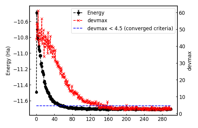
turbogenius vmcopt -post -optwarmup 80 -plot

Check plot_energy_and_devmax.png and the files in the parameters_graphs directory.

../../../_images/plot_energy_and_devmax.png

04 JDFT ansatz - VMC 

The next step is to run a single-shot VMC calculation. This is done using the vmc module of TurboGenius. First, prepare the wavefunction and pseudopotential files:

cd ../04_vmc/
cp ../03_optimization/fort.10 fort.10
cp ../03_optimization/pseudo.dat .

Next, generate an input file datasvmc.input using:

turbogenius vmc -g -steps 1000 -nw 128

Then, run the VMC calculation, e.g., by typing:

TURBOVMC_RUN_COMMAND="mpirun -np 16 turborvb-mpi.x"
export TURBOVMC_RUN_COMMAND

turbogenius vmc -r

Finally, run the postprocess:

turbogenius vmc -post -bin 10 -warmup 3

Check the reblocked total energy and error in the file pip0.d.

05 JDFT ansatz - LRDMC 

Now we proceed to the lattice regularized diffusion Monte Carlo calculation that can improve a trial wavefunction obtained by a DFT calculation or a VMC optimization. One should refer to the Hydrogen tutorial for the details.

In this section, we will perform the calculation at the lattice constant alat=0.20. First, copy the prepared wavefunction and the pseudopotential files:

# LRDMC run
cd ../05_lrdmc/alat_0.20/
cp ../../04_vmc/fort.10 .
cp ../../04_vmc/pseudo.dat .

Next, generate an input file datasfn.input for the LRDMC calculation:

turbogenius lrdmc -g -etry -11.70 -alat -0.20 -steps 1000 -nw 128

Then, run the calculation by typing:

TURBOVMC_RUN_COMMAND="mpirun -np 16 turborvb-mpi.x"
export TURBOVMC_RUN_COMMAND

turbogenius lrdmc -r

Finally, run the postprocess:

turbogenius lrdmc -post -bin 20 -corr 3 warmup 5

We will get E at a=0.20 bohr in pip0_fn.d.

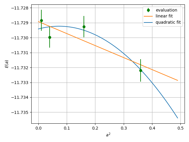
One then follows the above procedure for several choices of alat, and extrapolates the energy value at \(a \to 0\). See the Hydrogen tutorial for the concrete steps.

../../../_images/lrdmc_extrapolation.png

06 Summary 

The total energy obtained at the steps above and the reference value are summarized as follows:

DFT (LDA) = -11.4591 Ha
VMC (JDFT) = -11.7042(4) Ha
LRDMC (JDFT at a=0.20 bohr) = -11.7289(6) Ha.
LRDMC (JDFT extrapolated to a \(\to 0\)) = -11.7289(5) Ha.