02Carbon_dimer
00 Introduction
From this tutorial, you can learn how to calculate all-electron Variational Monte Carlo (VMC) and lattice regularized diffusion Monte Carlo (LRDMC) energies of the C2 dimer with various ansatz. JDFT, JSD, JsAGPs, JAGPu, and JAGP (JPf) with turbo-genius. You can download all the input and output files for this tutorial from here.
- C2 dimer
Ebond = 6.44 eV = 148.508 kcal/mol = 0.236 Ha J. Chem. Theory Comput. 16, 6114-6131 (2020)
dC-C = 2.3481 bohr J. Chem. Phys. 128, 174101 (2008)
Warning
In this tutorial, dC-C = 2.300 bohr is used just for simplicity. So, please change it if you need a more accurat result.
01 C2 dimer and C atom - JDFT ansatz
01-01 Preparing a trial wave function
Download C2 dimer and C atom structures, C2.xyz.
# C2-dimer
2
comment line
C 0.0000 0.0000 -0.60855355000000000000
C 0.0000 0.0000 0.60855355000000000000

# C-atom
1
comment line
C 0.0000 0.0000 0.0000
# C2 dimer
cd 01JDFT/01C2_dimer/01trial_wavefunction/00makefort10
turbogenius makefort10 -g -str C2.xyz -detbasis vtz -jasbasis vdz -pp BFD

# C atom
cd 01JDFT/02C_atom/01trial_wavefunction/00makefort10
turbogenius makefort10 -g -str C.xyz -detbasis vtz -jasbasis vdz -pp BFD -neldiff 2
01-02 Generating a JAGPs template
One can generate a JAGPs template using the prepared makefort10.input by typing:
turbogenius makefort10 -r         # ``-r`` for running calculations
turbogenius makefort10 -post      # ``-post`` for post-analysis or cleanup
or
turbogenius makefort10 -r -post
01-03 Generating a Pseudo potential file
The pseudo potential file has been automatically generated by turbogenius.
%cat pseudo.dat
ECP
        1   1.87000000000000                2
        1           3
22.5516419100000        2.00000000000000        5.02991637000000
4.00000000000000        1.00000000000000        8.35973821000000
33.4389528500000        3.00000000000000        4.48361888000000
-19.1753732300000        2.00000000000000        3.93831258000000
        2   1.87000000000000                2
        1           3
22.5516419100000        2.00000000000000        5.02991637000000
4.00000000000000        1.00000000000000        8.35973821000000
33.4389528500000        3.00000000000000        4.48361888000000
-19.1753732300000        2.00000000000000        3.93831258000000
01-04 Adding molecular orbitals to the JAGPs template
One should convert the generated JAGPs template to Jastrow Slater Determinant (JSD) one to prepare a trial wavefunction using DFT. This can be done using the convertfort10 module. Generate an input file for convertfort10mol using:
mv fort.10 fort.10_in
turbogenius convertfort10mol -g
After preparing convertfort10mol.input, run the calculation by typing the following commands to covert fort.10_in (JAGPs) to fort.10_new (JSD) by:
turbogenius convertfort10mol -r
turbogenius convertfort10mol -post
01-05 Run DFT
As written above, the coefficients of the molecular orbitals generated by convertfort10mol.x are random. Therefore, the next step is to optimize the coefficients using a build-in DFT code, called prep.x. This is done by using the prep module of Turbo-Genius.
Move to a working directory:
cd ../01DFT
Next, copy the prepared fort.10 and pseudo.dat to 01DFT directory:
cp ../00makefort10/fort.10 ./
cp ../00makefort10/pseudo.dat ./
To generate an input file for a DFT calculation type the following command:
# for C2 molecule
turbogenius prep -g -grid 0.10 0.10 0.10 -lbox 12.0 12.0 14.0

# for C atom
turbogenius prep -g -grid 0.10 0.10 0.10 -lbox 12.0 12.0 12.0
Note
In the generated prep.input file, set nelocc to 4. The occupation of the orbitals is specified at the end of the input file (2 in this case, indicating paired electrons)
Launch the DFT job.
# on a local machine (serial version)
prep-serial.x < prep.input > out_prep
# on a local machine (parallel version)
mpirun -np XX prep-mpi.x < prep.input > out_prep
# on a cluster machine (PBS)
qsub submit.sh
# on a cluster machine (Slurm)
sbatch submit.sh
Check the convergence.
turbogenius prep -post

grep Iter out_prep
Iter,E,xc,corr     1       -13.1203443        -3.6300842        -0.4666827        19.4803860
Iter,E,xc,corr     2       -11.9869924        -2.0332673        -0.3526467         1.1333519
Iter,E,xc,corr     3       -11.2327951        -2.3881088        -0.3788108         0.7541973
Iter,E,xc,corr     4       -20.6331707        -1.9842066        -0.4019725         9.4003755
Iter,E,xc,corr     5       -11.3440293        -2.3325513        -0.3733283         9.2891413
Iter,E,xc,corr     6       -11.0026202        -2.6778705        -0.4050588         0.3414091
Iter,E,xc,corr     7       -11.0245545        -2.5463056        -0.3964621         0.0219343
Iter,E,xc,corr     8       -10.9915229        -2.6421696        -0.4050391         0.0330315
Iter,E,xc,corr     9       -10.9894860        -2.6702884        -0.4084529         0.0020369
Iter,E,xc,corr    10       -10.9899084        -2.6757655        -0.4102938         0.0004223
# Iterations =    10
01-06 Jastrow factor optimization (WF=JDFT)
One should refer to the Hydrogen tutorial for the details. Here, only the commands are shown.
cd ../../02optimization/
cp ../01trial_wavefunction/01DFT/fort.10_new fort.10
cp ../01trial_wavefunction/01DFT/pseudo.dat ./
cp fort.10 fort.10_dft
turbogenius vmcopt -g -opt_onebody -opt_twobody -opt_jas_mat -optimizer lr -vmcoptsteps 100 -steps 400
Run the optimization jobs.
# on a local machine (serial version)
turborvb-serial.x < datasmin.input > out_min
# on a local machine (parallel version)
mpirun -np XX turborvb-mpi.x < datasmin.input > out_min
# on a cluster machine (PBS)
qsub submit.sh
# on a cluster machine (Slurm)
sbatch submit.sh
Check the convergence.
turbogenius vmcopt -post -optwarmup 80 -plot
# and then please follow the instructions.
01-07 VMC (WF=JDFT)
Please refer to the Hydrogen tutorial for the details. Here, only needed commands are shown.
cd ../03vmc/
cp ../02optimization/fort.10 fort.10
cp ../02optimization/pseudo.dat .
turbogenius vmc -g
vi datasvmc.input # if needed

# on a local machine (serial version)
turborvb-serial.x < datasvmc.input > out_vmc
# on a local machine (parallel version)
mpirun -np XX turborvb-mpi.x < datasvmc.input > out_vmc
# on a cluster machine (PBS)
qsub submit.sh
# on a cluster machine (Slurm)
sbatch submit.sh

turbogenius vmc -post -bin 10 -warmup 5
You may obtain like:
# C2-dimer
% cat pip0.d
number of bins read =         996
Energy =  -11.0221801195572       2.314058967237164E-004
Variance square =  0.225404174390588       6.661308870842383E-004
Est. energy error bar =  2.326984685231173E-004  5.429092343987092E-006
Est. corr. time  =   1.53214388283156       7.133083209261912E-002

# C-atom
% cat pip0.d
number of bins read =         999
Energy =  -5.40965078208914       1.502837476823764E-004
Variance square =  8.609101949646993E-002  3.231616256487902E-004
Est. energy error bar =  1.528893139652585E-004  3.472140401553639E-006
Est. corr. time  =   1.73685872518992       7.845390460943868E-002
01-08 LRDMC (WF=JDFT)
One should refer to the Hydrogen tutorial for the details. Here, only needed explanations and commands are shown.
Run LRDMC jobs for each alat:
cd ../04lrdmc/alat_0.XX/

# for each alat
cp ../../03vmc/fort.10 ./
cp ../../03vmc/pseudo.dat .

# C2 molecule
turbogenius lrdmc -g -etry -11.00 -alat -0.XX

# C atom
turbogenius lrdmc -g -etry -5.00 -alat -0.XX

# on a local machine (serial version)
turborvb-serial.x < datasfn.input > out_fn
# on a local machine (parallel version)
mpirun -np XX turborvb-mpi.x < datasfn.input > out_fn # parallel version
# on a cluster machine (PBS)
qsub submit.sh
# on a cluster machine (Slurm)
sbatch submit.sh

turbogenius lrdmc -bin 20 -corr 3 warmup 5
Extrapolation:
alat_list="0.10 0.20 0.30 0.40"
lrdmc_root_dir=`pwd`

num=0
echo -n > ${lrdmc_root_dir}/evsa.gnu
for alat in $alat_list
do
    cd alat_${alat}
    turbo-genius.sh -j lrdmc -post -eq 5 -reb 20 -col 5
    num=`expr ${num} + 1`
    echo -n "${alat} " >> ${lrdmc_root_dir}/evsa.gnu
    grep "Energy =" pip0_fn.d  | awk '{print $3, $4}' >> ${lrdmc_root_dir}/evsa.gnu
    cd ${lrdmc_root_dir}
done

# quartic fit (C2 dimer)
# please replace sed with gsed on Mac
sed "1i 2  ${num}  4  1" evsa.gnu > evsa.in
funvsa.x < evsa.in > evsa.out

# quadratic fit (C atom)
# please replace sed with gsed on Mac
sed "1i 1  ${num}  4  1" evsa.gnu > evsa.in
funvsa.x < evsa.in > evsa.out

# plot
gnuplot
p "evsa.gnu" u 1:2:3 with yerr
It performs curve fitting for energies vs alat, which is then used for extrapolation. While running turbo-genius asks for the degree of polynomial to be used for curve fitting. The result of fitting is written to the file evsa.out
For quartic fitting i.e. E(a)=E(0) + k_{1} \cdot a^2 + k_{2} \cdot a^4, the results are like:
# C2 dimer
% cat evsa.out
Reduced chi^2  =   3.24139195024559
Coefficient found
1  -11.0529822174764       1.886835280808058E-004  <- E_0
2 -3.752828455181791E-003  3.868657694133935E-003  <- k_1
3 -2.343738962778753E-002  1.487080872118977E-002  <- k_2
For quadratic fitting i.e. E(a)=E(0) + k_{1} \cdot a^2, the results are like:
# C atom
% cat evsa.out
Reduced chi^2  =   3.22600367069279
Coefficient found
1 -5.42188811770239        1.033538868667457E-004  <- E_0
2 -3.493534258715859E-003  7.118635862498798E-004  <- k_1
Finally:
C2 dimer
VMC(JDFT) = -11.02218(23) Ha
LRDMC(JDFT) = -11.05298(19) Ha
C atom
VMC(JDFT) = -5.40965(15) Ha
LRDMC(JDFT) = -5.42189(10) Ha
Binding energy
Ebond = 0.2028(3) Ha = 5.51(8) eV (VMC-JDFT)
Ebond = 5.656(3) eV (DMC-JDFT) (J. Chem. Phys. 2008, 128, 174101 ).
Ebond = 0.2092(2) Ha = 5.69(5) eV (LRDMC-JDFT)
Ebond = 0.236 Ha = 6.44 eV (Experiment)
02 C2 dimer and C atom - JsAGPs ansatz
02-01 Conversion of WF (WF=JsAGPs)
The procedure is the almost same as in the Hydrogen-dimer tutorial.
Three hybrid-orbitals (nhyb=4) were employed here.
Please refer to the Hydrogen tutorial for the details.
# C2-dimer/copy wfs
cd ../../../03JsAGPs/01C2_dimer/01convert_WF_JSD_to_JAGP/
cp ../../../01JDFT/01C2_dimer/03vmc/fort.10 ./fort.10
cp ../../../01JDFT/01C2_dimer/03vmc/pseudo.dat .

# C atom/copy wfs
cd ../../../03JsAGPs/02C_atom/01_01convert_WF_JSD_to_JAGP/
cp ../../../01JDFT/02C_atom/03vmc/fort.10 ./fort.10
cp ../../../01JDFT/02C_atom/03vmc/pseudo.dat .
#conversion (C2-dimer)
turbogenius convertwf -to agps -nosym -hyb 4 4 # add hybrid orbitals 4 4 for the first and the second C atoms

#conversion (C atom)
turbogenius convertwf -to agps -nosym # hybrid orbitals are added later. See below
# grep Overlap out_conv
....
Overlap square with no zero  0.9999....
# correlated sampling
cp fort.10_bak ./fort.10_corr
turbogenius correlated-sampling -g

# on a local machine (serial version)
turborvb-serial.x < datasvmc.input > out_vmc
readforward-serial.x  < datasvmc.input > out_readforward
# on a local machine (parallel version)
mpirun -np XX turborvb-mpi.x < datasvmc.input > out_vmc
mpirun -np XX readforward-mpi.x < datasvmc.input > out_readforward
# on a cluster machine (PBS)
qsub submit.sh
# on a cluster machine (Slurm)
sbatch submit.sh

# check the overlap
%cat corrsampling.dat
                                Number of bins                 10
                    reference energy: E(fort.10)  -0.110045875E+02     0.252368934E-01
                reweighted energy: E(fort.10_corr)  -0.110045875E+02     0.252368985E-01
reweighted difference: E(fort.10)-E(fort.10_corr)   -0.148834687E-07     0.316227766E-07
        Overlap square : (fort.10,fort.10_corr)    0.999999998E+00     0.316227766E-07
The conversion procedure is a bit complicated for the C atom. You should optimize the matrix elements before adding hybrid orbitals.
cd ../01_02convert_WF_JSD_to_JAGP/
cp ../01_01convert_WF_JSD_to_JAGP/fort.10 .
cp ../01_01convert_WF_JSD_to_JAGP/pseudo.dat .
turbogenius vmcopt -g -opt_onebody -opt_twobody -opt_jas_mat -opt_det_mat -optimizer lr

# on a local machine (serial version)
turborvb-serial.x < datasmin.input > out_min
# on a local machine (parallel version)
mpirun -np XX turborvb-mpi.x < datasmin.input > out_min
# on a cluster machine (PBS)
qsub submit.sh
# on a cluster machine (Slurm)
sbatch submit.sh
Finally, you can convert the optimized WF to the JAGP one with -hyb 4.
#conversion with 4 hybrid orbitals
turbogenius convertwf -to agps -nosym -hyb 4
Please check if the largest eigenvalues are non zero that were zero before the optimization.
% cat out_conv
...
41 0.359417387280524595E-01
42 0.472612394607655972         <- here
43 50.2735591956323731          <- here
44 52.3040643927227791          <- here
45 52.4454593457030782          <- here
dimension =          45           4
dimension =          45           4
dimension =          45           4
dimension =          45           4
Please check the energy diff. by the correlated sampling.
# correlated sampling
cp fort.10_bak ./fort.10_corr
turbogenius correlated-sampling -g

# on a local machine (serial version)
turborvb-serial.x < datasvmc.input > out_vmc
readforward-serial.x  < datasvmc.input > out_readforward
# on a local machine (parallel version)
mpirun -np XX turborvb-mpi.x < datasvmc.input > out_vmc
mpirun -np XX readforward-mpi.x < datasvmc.input > out_readforward
# on a cluster machine (PBS)
qsub submit.sh
# on a cluster machine (Slurm)
sbatch submit.sh
02-02 VMC-optimization (WF=JsAGPs)
Please refer to the Hydrogen tutorial for the details. Here, only the commands are shown.
# for C2 dimer
cd ../02optimization/
cp ../01convert_WF_JSD_to_JAGP/fort.10 fort.10
cp ../01convert_WF_JSD_to_JAGP/pseudo.dat pseudo.dat
cp fort.10 fort.10_jdft
turbogenius vmcopt -g -opt_onebody -opt_twobody -opt_jas_mat -opt_det_mat -optimizer lr

# for C atom
cd ../02optimization/
cp ../01_02convert_WF_JSD_to_JAGP/fort.10 fort.10
cp ../01_02convert_WF_JSD_to_JAGP/pseudo.dat pseudo.dat
cp fort.10 fort.10_jdft
turbogenius vmcopt -g -opt_onebody -opt_twobody -opt_jas_mat -opt_det_mat -optimizer lr
Run a optimization job.
# on a local machine (serial version)
turborvb-serial.x < datasmin.input > out_min
# on a local machine (parallel version)
mpirun -np XX turborvb-mpi.x < datasmin.input > out_min
# on a cluster machine (PBS)
qsub submit.sh
# on a cluster machine (Slurm)
sbatch submit.sh
Check the convergence.
turbogenius vmcopt -post -optwarmup 100 -plot
# and then please follow the instructions.
02-03 VMC (WF=JsAGPs)
Please refer to the Hydrogen tutorial for the details. Here, only needed commands are shown.
cd ../03vmc
cp ../02optimization/fort.10 ./fort.10
cp ../02optimization/pseudo.dat .
turbogenius vmc -g

# on a local machine (serial version)
turborvb-serial.x < datasvmc.input > out_vmc
# on a local machine (parallel version)
mpirun -np XX turborvb-mpi.x < datasvmc.input > out_vmc
# on a cluster machine (PBS)
qsub submit.sh
# on a cluster machine (Slurm)
sbatch submit.sh

turbogenius vmc -post -bin 10 -warmup 5
You may obtain:
# C2 dimer
% cat pip0.d
number of bins read =         499
Energy =  -11.0561023752813       2.657081737992969E-004
Variance square =  0.167151337506581       2.487175392299656E-003
Est. energy error bar =  2.667881948465201E-004  9.740755305129974E-006
Est. corr. time  =   1.36165378936245       9.657211844194399E-002

# C2 dimer
% cat pip0.d
number of bins read =         499
Energy =  -5.42023281231657       1.747843070690741E-004
Variance square =  6.151263349430580E-002  2.812473020121101E-004
Est. energy error bar =  1.823230486819808E-004  5.739947472392408E-006
Est. corr. time  =   1.72750276011311       0.107600086165112
02-04 LRDMC (WF=JsAGPs)
Please refer to the Hydrogen tutorial for the details. Here, only the commands are shown.
cd ../04lrdmc/alat_0.XX/

# for each alat
cp ../../03vmc/fort.10 ./
cp ../../03vmc/pseudo.dat .

# C2 molecule
turbogenius lrdmc -g --help -etry -11.00 -alat -0.XX

# C atom
turbogenius lrdmc -g --help -etry -5.00 -alat -0.XX

# on a local machine (serial version)
turborvb-serial.x < datasfn.input > out_fn
# on a local machine (parallel version)
mpirun -np XX turborvb-mpi.x < datasfn.input > out_fn # parallel version
# on a cluster machine (PBS)
qsub submit.sh
# on a cluster machine (Slurm)
sbatch submit.sh

turbogenius lrdmc -bin 20 -corr 3 warmup 5
Extrapolation:
alat_list="0.10 0.20 0.30 0.40"
lrdmc_root_dir=`pwd`

num=0
echo -n > ${lrdmc_root_dir}/evsa.gnu
for alat in $alat_list
do
    cd alat_${alat}
    turbo-genius.sh -j lrdmc -post -eq 5 -reb 20 -col 5
    num=`expr ${num} + 1`
    echo -n "${alat} " >> ${lrdmc_root_dir}/evsa.gnu
    grep "Energy =" pip0_fn.d  | awk '{print $3, $4}' >> ${lrdmc_root_dir}/evsa.gnu
    cd ${lrdmc_root_dir}
done

# quartic fit (C2 dimer)
# please replace sed with gsed on Mac
sed "1i 2  ${num}  4  1" evsa.gnu > evsa.in
funvsa.x < evsa.in > evsa.out

# quadratic fit (C atom)
# please replace sed with gsed on Mac
sed "1i 1  ${num}  4  1" evsa.gnu > evsa.in
funvsa.x < evsa.in > evsa.out

# plot
gnuplot
p "evsa.gnu" u 1:2:3 with yerr
# C2 dimer
Reduced chi^2  =  0.211949768672111
Coefficient found
        1  -11.0749244254452       1.269668477442219E-004
        2 -5.572540169827904E-003  8.734350696222097E-004

# C atom
Reduced chi^2  =   1.48922837922392
Coefficient found
        1  -5.42734029684322       8.031603687503355E-005
        2 -1.750555796426137E-003  5.639930126170355E-004
Finally:
C2 dimer
VMC(JsAGPs) = -11.05610(27) Ha
LRDMC(JsAGPs) = -11.07492(13) Ha
C atom
VMC(JsAGPs) = -5.4202(17) Ha
LRDMC(JsAGPs) = -5.42734(8) Ha
Binding energy
Ebond = 0.2028(3) Ha = 5.519(8) eV (VMC-JDFT)
Ebond = 0.2157(4)Ha = 5.870(10) eV (VMC-JsAGPs)
Ebond = 5.656(3) eV (DMC-JDFT) (J. Chem. Phys. 2008, 128, 174101 ).
Ebond = 0.2092(2) Ha = 5.693(5) eV (LRDMC-JDFT)
Ebond = 0.2202(2)Ha = 5.993(5)eV (LRDMC-JsAGPs)
Ebond = 0.236 Ha = 6.44 eV (Experiment)
03 C2 dimer and C atom - JAGPu ansatz
03-01 prepration of a wave function
You can convert the JAGPs WF to the JAGPu WF by the following commands
# C2 dimer
cd ../../../04JAGPu/01C2_dimer/01trial_wavefunction/01DFT/
cp ../../../../03JsAGPs/01C2_dimer/03vmc/fort.10 .
cp ../../../../03JsAGPs/01C2_dimer/03vmc/pseudo.dat .
turbogenius convertwf -to agpu -nosym

# add molecular orbital (i.e., JAGPu -> JSD)
turbogenius convertwf -to sd
03-02 Generate a trial wave function using DFT with a magnetic moment (C2 dimer:).
The next step is to prepare a trial wave function using the built-in DFT code. Here you can set magnetic moments on each atom to obtain an AFM initial state.
# both for C2 dimer and C atom
cd ../01DFT

#C2-dimer
turbogenius prep -g -xc lsda -f 0.01 -grid 0.10 0.10 0.10 -lbox 12.0 12.0 14.0 -m u d
#C-atom
turbogenius prep -g -xc lsda -f 0.01 -grid 0.10 0.10 0.10 -lbox 12.0 12.0 12.0 -m u
Then, you can run DFT by typing:
# on a local machine (serial version)
prep-serial.x < prep.input > out_prep
# on a local machine (parallel version)
mpirun -np XX prep-mpi.x < prep.input > out_prep
# on a cluster machine (PBS)
qsub submit.sh
# on a cluster machine (Slurm)
sbatch submit.sh

turbogenius prep -post
03-03 Check local magnetic moments (C2 dimer)
You can check the obtained magnetic moments by using plot_orbitals.x
# copy fort.10
cd ../02check_magnetization
cp ../01DFT/pseudo.dat .

# plot spin density
cp ../01DFT/fort.10_new fort.10
plot_orbitals.x

Number of molecular orbitals :            6
Choose box size (x,y,z)
15 15 15
15.0000000000000        15.0000000000000        15.0000000000000
Choose number of mesh points (x,y,z) :
61 61 61
61          61          61
Choose orbitals to tabulate (possible answers all, partial, charge, spin) :
spin
spin
Please give  the lowest molecular orbital within 1 and            8
1
Number of fully occupied molecular orbital/total number occupied by up and down?
4 4
Momentum magnetization ? (unit 2pi/cellscale)
0 0 0

You obtain output_spin000000.xsf. You can depict it using xcrysden:
xcrysden --xsf output_spin000000.xsf
open -a output_spin000000.xsf  # e.g., VESTA
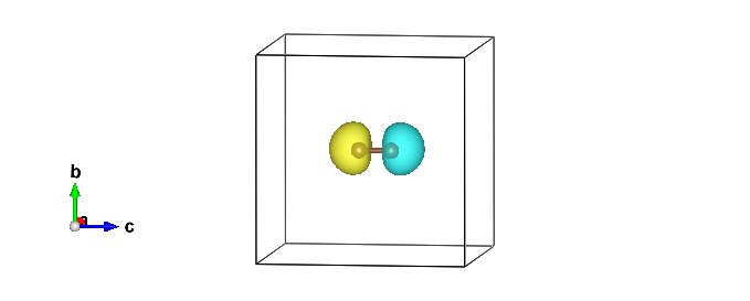
Thus, one can obtain an AFM trial wavefunction.
03-04 Convert JDFT WF to JAGPu one
Next step is to convert the optimized JDFT WF to a JAGPu one. You should check the consistency after conversion.
# C2-dimer
# conversion of WF (02convert_WF_JDFT_to_JAGP)
cd ../../02convert_WF_JDFT_to_JAGP/
cp ../01trial_wavefunction/01DFT/fort.10_new fort.10
cp ../01trial_wavefunction/01DFT/pseudo.dat .

#conversion (C2-dimer)
turbogenius convertwf -to agpu -nosym -hyb 4 4 # add hybrid orbitals 4 4 for the first and the second C atoms

#conversion (C atom)
turbogenius convertwf -to agpu -nosym # hybrid orbitals are added later. See below
# grep Overlap out_conv
....
Overlap square with no zero  0.9999....
# correlated sampling
cp fort.10_bak ./fort.10_corr
turbogenius correlated-sampling -g

# on a local machine (serial version)
turborvb-serial.x < datasvmc.input > out_vmc
readforward-serial.x  < datasvmc.input > out_readforward
# on a local machine (parallel version)
mpirun -np XX turborvb-mpi.x < datasvmc.input > out_vmc
mpirun -np XX readforward-mpi.x < datasvmc.input > out_readforward
# on a cluster machine (PBS)
qsub submit.sh
# on a cluster machine (Slurm)
sbatch submit.sh

# check the overlap
%cat corrsampling.dat
# Here, you may loose ~ 100mHa for the C2 dimer.
Warning
You should use more hybrid orbitals in a real research project! (e.g. ~ 7).
The conversion procedure is again complicated for the C atom. Please do the same procedure as in the JAGPs case.
03-05 Optimization (WF=JAGPu)
Now that you have obtained a good trial JAGPu wavefunction, you can optimize its nodal surface at the VMC level.
#C2 dimers
cd ../03optimization/
cp ../02convert_WF_JDFT_to_JAGP/fort.10 fort.10
cp ../02convert_WF_JDFT_to_JAGP/pseudo.dat ./
cp fort.10 fort.10_jdft
turbogenius vmcopt -g -opt_onebody -opt_twobody -opt_jas_mat -opt_det_mat -optimizer lr

#C atom
cd ../03optimization/
cp ../02_02convert_WF_JDFT_to_JAGP/fort.10 fort.10
cp ../02_02convert_WF_JDFT_to_JAGP/pseudo.dat ./
cp fort.10 fort.10_jdft
turbogenius vmcopt -g -opt_onebody -opt_twobody -opt_jas_mat -opt_det_mat -optimizer lr
Run VMC-opt runs
# on a local machine (serial version)
turborvb-serial.x < datasmin.input > out_min
# on a local machine (parallel version)
mpirun -np XX turborvb-mpi.x < datasmin.input > out_min
# on a cluster machine (PBS)
qsub submit.sh
# on a cluster machine (Slurm)
sbatch submit.sh

#average fort.10
turbogenius vmcopt -post -optwarmup 100 -plot
03-06 VMC and LRDMC
VMC and LRDMC procesures are the same as in the JsAGPs case.
# VMC
cd ../04vmc
cp ../03optimization/fort.10 ./fort.10
cp ../03optimization/pseudo.dat .
turbogenius vmc -g

# on a local machine (serial version)
turborvb-serial.x < datasvmc.input > out_vmc
# on a local machine (parallel version)
mpirun -np XX turborvb-mpi.x < datasvmc.input > out_vmc
# on a cluster machine (PBS)
qsub submit.sh
# on a cluster machine (Slurm)
sbatch submit.sh

turbogenius vmc -post -bin 10 -warmup 5
# C2-dimer
% cat pip0.d
number of bins read =         499
Energy =  -11.0639657131521       2.451753146145206E-004
Variance square =  0.144445612617421       1.504179616851022E-003
Est. energy error bar =  2.382267038858785E-004  7.075164804881710E-006
Est. corr. time  =   1.25601105010529       7.608951964475108E-002

# C atom
% cat pip0.d
number of bins read =         499
Energy =  -5.42587679977424       1.407145615635295E-004
Variance square =  4.092231745300601E-002  3.752942906547522E-004
Est. energy error bar =  1.386833646006721E-004  4.181441619092614E-006
Est. corr. time  =   1.50231356841123       8.930286017090674E-002
Heres are commands for LRDMCs.
cd ../04lrdmc/alat_0.XX/

# for each alat
cp ../../03vmc/fort.10 ./
cp ../../03vmc/pseudo.dat .

# C2 molecule
turbogenius lrdmc -g --help -etry -11.00 -alat -0.XX

# C atom
turbogenius lrdmc -g --help -etry -5.00 -alat -0.XX

# on a local machine (serial version)
turborvb-serial.x < datasfn.input > out_fn
# on a local machine (parallel version)
mpirun -np XX turborvb-mpi.x < datasfn.input > out_fn # parallel version
# on a cluster machine (PBS)
qsub submit.sh
# on a cluster machine (Slurm)
sbatch submit.sh

turbogenius lrdmc -bin 20 -corr 3 warmup 5
# extrapolation
alat_list="0.10 0.20 0.30 0.40 0.50"
lrdmc_root_dir=`pwd`

num=0
echo -n > ${lrdmc_root_dir}/evsa.gnu
for alat in $alat_list
do
    cd alat_${alat}
    turbo-genius.sh -j lrdmc -post -eq 5 -reb 20 -col 5
    num=`expr ${num} + 1`
    echo -n "${alat} " >> ${lrdmc_root_dir}/evsa.gnu
    grep "Energy =" pip0_fn.d  | awk '{print $3, $4}' >> ${lrdmc_root_dir}/evsa.gnu
    cd ${lrdmc_root_dir}
done

# quadratic fit
# please replace sed with gsed on Mac
sed "1i 2  ${num}  4  1" evsa.gnu > evsa.in
funvsa.x < evsa.in > evsa.out
# C2 dimer
Reduced chi^2  =  0.229533908546215
Coefficient found
        1  -11.0757437909485       1.464579638032684E-004
        2 -1.087864661257017E-002  2.922117199514128E-003
        3  6.078076478538951E-003  1.109481138283852E-002

# C atom
Reduced chi^2  =  3.354870888922901E-003
Coefficient found
        1  -5.42939660705427       7.390966338489803E-005
        2 -1.281854484441583E-003  1.529393458975311E-003
        3 -5.479765301310381E-003  5.869251318513092E-003
Finally:
C2 dimer
VMC(JAGPu) = -11.06397(25) Ha
LRDMC(JAGPu) = -11.07574(15) Ha
C atom
VMC(JAGPu) = -5.42588(14) Ha
LRDMC(JAGPu) = -5.42940(7)Ha
Binding energy
Ebond = 0.2028(3) Ha = 5.519(8) eV (VMC-JDFT)
Ebond = 0.2157(4) Ha = 5.870(10) eV (VMC-JsAGPs)
Ebond = 0.2122(4) Ha = 5.774(10) eV (VMC-JAGPu)
Ebond = 5.656(3) eV (DMC-JDFT) (J. Chem. Phys. 2008, 128, 174101 ).
Ebond = 0.2092(2) Ha = 5.693(5) eV (LRDMC-JDFT)
Ebond = 0.2202(2) Ha = 5.993(5) eV (LRDMC-JsAGPs)
Ebond = 0.2169(2) Ha = 5.903(5) eV (LRDMC-JAGPu)
Ebond = 0.236 Ha = 6.44 eV (Experiment)
04 C2 dimer and C atom - JAGP (JPf) ansatz
The most important procedure in a Pfaffian calculation is to convert a JDFT or JAGPu ansatz to JAGP(JPf) ansatz. Since the JAGP ansatz is a special case of the JPf one, where only G_{ud} and G_{du} terms are defined as described in the section review paper, the conversion can be realized just by direct substitution. Therefore, the main challenge is to find a reasonable initialization for the two spin-triplet sectors G_{uu} and G_{dd} that are not described in the JAGP and that otherwise have to be set to 0.
There are two possible approaches to convert an ansatz: \rm(\hspace{.18em}i\hspace{.18em}) for polarized systems, we can build the G_{uu} block of the matrix by using an even number of \{ \phi_i\} and build an antisymmetric g_{uu}, where the eigenvalues \lambda_k are chosen to be large enough to occupy certainly these unpaired states, as in the standard Slater determinant used for our initialization.
Again, we emphasize that this works only for polarized systems. \rm(\hspace{.08em}ii\hspace{.08em}) The second approach that also works in a spin-unpolarized case is to determine a standard broken symmetry single determinant ansatz ({it e.g.}, by TurboRVB built-in DFT within the LSDA) and modify it with a global spin rotation. Indeed, in the presence of finite local magnetic moments, it is often convenient to rotate the spin moments of the WF in a direction perpendicular to the spin quantization axis chosen for our spin-dependent Jastrow factor, {it i.e.}, the z quantization axis. In this way one can obtain reasonable initializations for G_{uu} and G_{dd}. TurboRVB allows every possible rotation, including an arbitrary small one close to the identity. A particularly important case is when a rotation of \pi/2 is applied around the y direction. This operation maps |\uparrow \rangle \rightarrow \frac{1} {\sqrt{2}} \left( | \uparrow \rangle + |\downarrow \rangle \right) \mbox{ and } |\downarrow \rangle \rightarrow \frac 1 {\sqrt{2}} \left( | \uparrow \rangle - |\downarrow \rangle \right). One can convert from a AGP the pairing function that is obtained from a VMC optimization {g_{ud}}(\mathbf{i},\mathbf{j}) = {f_S}({{\mathbf{r}}_i},{{\mathbf{r}}_j})\frac{{\left| { \uparrow \downarrow } \right\rangle - \left| { \downarrow \uparrow } \right\rangle }}{{\sqrt 2 }} + {f_T}({{\mathbf{r}}_i},{{\mathbf{r}}_j})\frac{{\left| { \uparrow \downarrow } \right\rangle + \left| { \downarrow \uparrow } \right\rangle }}{{\sqrt 2 }} to a Pf one {g_{ud}}(\mathbf{i},\mathbf{j}) \to g\left( {\mathbf{i},\mathbf{j}} \right){\text{ }} = {f_S}({{\mathbf{r}}_i},{{\mathbf{r}}_j})\frac{{\left| { \uparrow \downarrow } \right\rangle - \left| { \downarrow \uparrow } \right\rangle }}{{\sqrt 2 }} + {f_T}({{\mathbf{r}}_i},{{\mathbf{r}}_j})\left( {\left| { \uparrow \uparrow } \right\rangle - \left| { \downarrow \downarrow } \right\rangle } \right). This transformation provides a meaningful initialization to the Pfaffian WF that can be then optimized for reaching the best possible description of the ground state within this ansatz.
The strategy \rm(\hspace{.08em}ii\hspace{.08em}) is employed for the C dimer (i.e., unpolarized case) while \rm(\hspace{.18em}i\hspace{.18em}) is employed for the C atom (i.e., polarized case)
04-01 (spin-singlet case) C2 dimer: Convert JAGPu WF to JAGP one
################
# C-dimer
################
cd ../../../05JAGP/01C2_dimer/01convert_WF_JAGPu_to_JAGP
cp ../../../04JAGPu/01C2_dimer/04vmc/fort.10 fort.10
cp ../../../04JAGPu/01C2_dimer/04vmc/pseudo.dat .

# convert to Paffian
turbogenius convertwf -to pf -rot 0.125 -nosym # pi/8 rotation

# correlated sampling
cp fort.10_bak ./fort.10_corr
turbogenius correlated-sampling -g

# on a local machine (serial version)
turborvb-serial.x < datasvmc.input > out_vmc
readforward-serial.x  < datasvmc.input > out_readforward
# on a local machine (parallel version)
mpirun -np XX turborvb-mpi.x < datasvmc.input > out_vmc
mpirun -np XX readforward-mpi.x < datasvmc.input > out_readforward
# on a cluster machine (PBS)
qsub submit.sh
# on a cluster machine (Slurm)
sbatch submit.sh

# check the overlap
# Here, you may loose some energy! because you have rotated the spins.
%cat corrsampling.dat
04-02 (spin-triplet case) C atom: Convert JAGPu WF to JAGP one
You can convert spin-polarized WFs using turbogenius in the same way as in the non spin-polarized WFs.
################
# C-dimer
################
cd ../../../05JAGP/02C_atom/01convert_WF_JAGPu_to_JAGP/
cp ../../../04JAGPu/02C_atom/02_02convert_WF_JDFT_to_JAGP/fort.10 .
cp ../../../04JAGPu/02C_atom/02_02convert_WF_JDFT_to_JAGP/pseudo.dat .

# convert to Paffian
turbogenius convertwf -to pf -rot 0.0

# correlated sampling
cp fort.10_bak ./fort.10_corr
turbogenius correlated-sampling -g

# on a local machine (serial version)
turborvb-serial.x < datasvmc.input > out_vmc
readforward-serial.x  < datasvmc.input > out_readforward
# on a local machine (parallel version)
mpirun -np XX turborvb-mpi.x < datasvmc.input > out_vmc
mpirun -np XX readforward-mpi.x < datasvmc.input > out_readforward
# on a cluster machine (PBS)
qsub submit.sh
# on a cluster machine (Slurm)
sbatch submit.sh

# check the overlap
%cat corrsampling.dat
04-03 VMC-opt, VMC and LRDMC
VMC and LRDMC procesures are the same as in the JsAGPs case.
#C2 dimers/vmcopt
cd ../03optimization/
cp ../02convert_WF_JAGPu_to_JAGP/fort.10 fort.10
cp ../02convert_WF_JAGPu_to_JAGP/pseudo.dat ./
cp fort.10 fort.10_jdft
turbogenius vmcopt -g -opt_onebody -opt_twobody -opt_jas_mat -opt_det_mat -optimizer lr

#C atom
cd ../03optimization/
cp ../02_02convert_WF_JAGPu_to_JAGP/fort.10 fort.10
cp ../02_02convert_WF_JAGPu_to_JAGP/pseudo.dat ./
cp fort.10 fort.10_jdft
turbogenius vmcopt -g -opt_onebody -opt_twobody -opt_jas_mat -opt_det_mat -optimizer lr

#C atom/vmcopt
# on a local machine (serial version)
turborvb-serial.x < datasmin.input > out_min
# on a local machine (parallel version)
mpirun -np XX turborvb-mpi.x < datasmin.input > out_min
# on a cluster machine (PBS)
qsub submit.sh
# on a cluster machine (Slurm)
sbatch submit.sh

#average fort.10
turbogenius vmcopt -post -optwarmup 100 -plot

# VMC
cd ../04vmc
cp ../03optimization/fort.10 ./fort.10
cp ../03optimization/pseudo.dat .
turbogenius vmc -g

# on a local machine (serial version)
turborvb-serial.x < datasvmc.input > out_vmc
# on a local machine (parallel version)
mpirun -np XX turborvb-mpi.x < datasvmc.input > out_vmc
# on a cluster machine (PBS)
qsub submit.sh
# on a cluster machine (Slurm)
sbatch submit.sh

turbogenius vmc -post -bin 10 -warmup 5

cd ../04lrdmc/alat_0.XX/

# for each alat
cp ../../04vmc/fort.10 ./
cp ../../04vmc/pseudo.dat .

# C2 molecule
turbogenius lrdmc -g --help -etry -11.00 -alat -0.XX

# C atom
turbogenius lrdmc -g --help -etry -5.00 -alat -0.XX

# on a local machine (serial version)
turborvb-serial.x < datasfn.input > out_fn
# on a local machine (parallel version)
mpirun -np XX turborvb-mpi.x < datasfn.input > out_fn # parallel version
# on a cluster machine (PBS)
qsub submit.sh
# on a cluster machine (Slurm)
sbatch submit.sh

turbogenius lrdmc -bin 20 -corr 3 warmup 5

# extrapolation
alat_list="0.10 0.20 0.30 0.40 0.50"
lrdmc_root_dir=`pwd`

num=0
echo -n > ${lrdmc_root_dir}/evsa.gnu
for alat in $alat_list
do
    cd alat_${alat}
    turbo-genius.sh -j lrdmc -post -eq 5 -reb 20 -col 5
    num=`expr ${num} + 1`
    echo -n "${alat} " >> ${lrdmc_root_dir}/evsa.gnu
    grep "Energy =" pip0_fn.d  | awk '{print $3, $4}' >> ${lrdmc_root_dir}/evsa.gnu
    cd ${lrdmc_root_dir}
done

# quadratic fit
# please replace sed with gsed on Mac
sed "1i 2  ${num}  4  1" evsa.gnu > evsa.in
funvsa.x < evsa.in > evsa.out
# C2 dimer
Reduced chi^2  =   1.02522438570479
Coefficient found
        1  -11.0850570018256       1.273076518444894E-004
        2 -5.555205897180920E-003  2.663590439241813E-003
        3 -6.811913435438424E-003  1.030873939747665E-002

# C atom
Reduced chi^2  =  6.175095826610375E-002
Coefficient found
        1  -5.42990249903405       7.249216286985208E-005
        2 -5.519306385371122E-003  1.468246248490263E-003
        3  1.078150972592802E-002  5.587021310029283E-003
Finally:
C2 dimer
VMC(JAGP) = -11.07452(24) Ha
LRDMC(JAGP) = -11.08506(12) Ha
C atom
VMC(JAGP) = -5.42700(15) Ha
LRDMC(JAGP) = -5.42990(72) Ha
Binding energy
Ebond = 0.2028(3) Ha = 5.519(8) eV (VMC-JDFT)
Ebond = 0.2157(4) Ha = 5.870(10) eV (VMC-JsAGPs)
Ebond = 0.2122(4) Ha = 5.774(10) eV (VMC-JAGPu)
Ebond = 0.2205(3) Ha = 6.000(8) eV (VMC-JAGP)
Ebond = 5.656(3) eV (DMC-JDFT) (J. Chem. Phys. 2008, 128, 174101 ).
Ebond = 0.2092(2) Ha = 5.693(5) eV (LRDMC-JDFT)
Ebond = 0.2202(2) Ha = 5.993(5) eV (LRDMC-JsAGPs)
Ebond = 0.2169(2) Ha = 5.903(5) eV (LRDMC-JAGPu)
Ebond = 0.2253(2) Ha = 6.130(5) eV (LRDMC-JAGP)
Ebond = 6.31(1) eV (LRDMC-JAGP, an optimized cc-pVTZ, all-electron) (J. Chem. Theory Comput. 16, 6114-6131 (2020)).
Ebond = 0.236 Ha = 6.44 eV (Experiment)