01Hydrogen_dimer

From this tutorial, you can learn how to calculate all-electron Variational Monte Carlo (VMC) and lattice regularized diffusion Monte Carlo (LRDMC) energies of the H₂ dimer using Turbo-genius. There is also a TurboRVB tutorial, which does the same calculations but without using Turbo-Genius. For detailed information about input parameters in various input files, we recomment visiting that tutorial. You can download all the input and output files for this tutorial from here.

00 Important introduction for TurboGenius

TurboGenius has a very useful command line tool that allows us to manipulate input and output files very efficiently. One of the most useful function of the command line tool is its helper. To see this, please try to type the following command:

% turbogenius --help
Usage: turbogenius [OPTIONS] COMMAND [ARGS]...

Options:
--help  Show this message and exit.

Commands:
convertfort10        convertfort10_genius
convertfort10mol     convertfort10mol_genius
convertpfaff         readforward_genius
convertwf            convert wavefunction
correlated-sampling  correlated_sampling_genius
lrdmc                lrdmc_genius
lrdmcopt             lrdmc_genius
makefort10           makefort10_genius
prep                 prep_genius
vmc                  vmc_genius
vmcopt               vmcopt_genius

You can easily see what commands are implemented in TurboGenius. Please type the following command to see what options are implemented for each command,

e.g., vmcopt:

% turbogenius vmcopt --help
Usage: turbogenius vmcopt [OPTIONS]

Options:
-post                 Postprocess
-r                    Run a program
-g                    Generate an input file
-vmcoptsteps INTEGER  Specify vmcoptsteps
-optwarmup INTEGER    Specify optwarmupsteps
-steps INTEGER        Specify steps per one iteration
-bin INTEGER          Specify bin_block
-warmup INTEGER       Specify warmupblocks
-nw INTEGER           Specify num_walkers
-maxtime INTEGER      Specify maxtime
-optimizer TEXT       Specify optimizer, sr or lr
-learn FLOAT          Specify learning_rate
-reg FLOAT            Specify regularization
-opt_onebody          flag for opt_onebody
-opt_twobody          flag for opt_twobody
-opt_det_mat          flag for opt_det_mat
-opt_jas_mat          flag for opt_jas_mat
-opt_det_basis_exp    flag for opt_det_basis_exp
-opt_jas_basis_exp    flag for opt_jas_basis_exp
-opt_det_basis_coeff  flag for opt_det_basis_coeff
-opt_jas_basis_coeff  flag for opt_jas_basis_coeff
-twist                flag for twist_average
-kpts INTEGER...      kpts, Specify Monkhorst-Pack grids and shifts,
                    [nkx,nky,nkz,kx,ky,kz]
-plot                 flag for plotting graph
-log TEXT             logger level, DEBUG, INFO, ERROR
--help                Show this message and exit.

e.g.,lrdmc

meiwaku20pc06% turbogenius lrdmc --help
Usage: turbogenius lrdmc [OPTIONS]

Options:
-post             Postprocess
-r                Run a program
-g                Generate an input file
-steps INTEGER    Specify lrdmcsteps
-bin INTEGER      Specify bin_block
-corr INTEGER     Specify correcting_factor
-alat FLOAT       Specify alat
-etry FLOAT       Specify etry
-warmup INTEGER   Specify warmupblocks
-nw INTEGER       Specify num_walkers
-maxtime INTEGER  Specify maxtime
-twist            flag for twist_average
-force            flag for force_calc_flag
-nonlocal TEXT    Specify nonlocalmoves, tmove, dla, dlatm
-log TEXT         logger level, DEBUG, INFO, ERROR
--help            Show this message and exit.

01 Preparing a JDFT trial wavefunction

01-01 Preparing a makefort10.input file

The first step of this tutorial is to generate an antisymmetrized Geminal Power (AGP) ansatz, which will be convert to a Slater determinant (SD) ansatz later. First, one should prepare makefort10.input to generate an AGP ansatz. The makefort10 module of Turbo-Genius can be used to generate AGP ansatz. Use the following command to generate a makefort10.input file. Remember that the structure file is also required at this step. Note: If you are interested in a pseudo-potential calculation, please refer to 02Carbon_dimer.

cd 01trial_wavefunction/00makefort10/
turbogenius makefort10 -g -str H2_dimer.xyz -detbasis cc-pVTZ -jasbasis cc-pVDZ -detcutbasis -jascutbasis

The command line options:

1. -j is used to specify the job type (like makefort10, prep etc.),

2. -g is used to generate input files. Alternatively -r may be used for running calculations and -post is used for postprocessing of results after running.

3. -str is used to indicate the structure file name, which could be in several formats: .xyz, .cif, POSCAR, .vasp, .xsf, or whatever ASE’s read function supports.

4. -detbasis is used to specify the basis set used to construct atomic orbitals for the determinant part. Here we are using cc-pVTZ type basis set to construct the atomic orbitals. See the –help for checking the basis set currently implemented.

5. --cutdetbasis flag is a command line argument to cut the determinant basis set based on the AZ algorithm (see below) It makes sense only for an all-electron calculation.

6. -jasbasis is used to specify the basis set used to construct atomic orbitals for the jastrow part. Here we are using cc-pVTZ type basis set to construct the atomic orbitals. See the –help for checking the basis set currently implemented.

7. --cutjasbasis flag is a command line argument to cut the determinant basis set based on the AZ algorithm (see below) It makes sense only for an all-electron calculation.

This is a generated makefort10.input.

# makefort10 input
&system
    posunits='bohr'
    natoms=2
    ntyp=1
    complexfort10=.false.
    pbcfort10=.false.
    yes_pfaff=.false.
    nxyz(1)=1
    nxyz(2)=1
    nxyz(3)=1
    phase(1)=0.0
    phase(2)=0.0
    phase(3)=0.0
    phasedo(1)=0.0
    phasedo(2)=0.0
    phasedo(3)=0.0
/

&electrons
    orbtype='normal'
    jorbtype='normal'
    twobody=-6
    filling='diagonal'
    yes_crystal=.false.
    yes_crystalj=.false.
    no_4body_jas=.true.
    neldiff=0
    !onebodypar=1.0
    twobodypar(1)=1.0
    !twobodypar=1.0
/

&symmetries
    nosym=.false.
    eqatoms=.true.
    rot_det=.true.
    symmagp=.true.
/

ATOMIC_POSITIONS
1.00000000  1.00000000  0.00000000000000  0.00000000000000  -0.70014352917385
1.00000000  1.00000000  0.00000000000000  0.00000000000000  0.70014352917385
/

ATOM_1
&shells
nshelldet=7
nshelljas=4
/
1   1   16
1   0.325800000000
1   1   16
1   5.095000000000
1   1   16
1   1.159000000000
1   1   16
1   0.102700000000
3   1   36
1   1.407000000000
3   1   36
1   0.388000000000
5   1   37
1   1.057000000000
# Parameters atomic Jastrow wf
1   1   16
1   1.962000000000
1   1   16
1   0.444600000000
1   1   16
1   0.122000000000
3   1   36
1   0.727000000000

Note

We have cut first few orbitals from the basis sets for atomic wavefunction as well as for the Jastrow part (nshelldet and nshelljas should be changed accordingly) by the option -cutbasis. The basis set can be automatically cut by using the --cutbasis flag as a command line argument while generating the makefort10 input. It cuts the basis set based on the AZ algorithm. An empirical criteria is \eta \ge 8 \times Z^2 in the s channel, where Z = \rm{atomic number}. For example, we can discard the topmost \eta = 33.87 \ge 8 \times 1^2. The cut s orbitals are implicitly compensated by the one body Jastrow term (See J. Chem. Theory Comput. 2019, 15, 7, 4044-4055 ).

For explanations of the input variables, please refer to the doc files in the TurboRVB repository.

Warning

If you want to use your own Det. or Jas. basis sets, you can edit makefort10.input at this step.

01-02 Generating a JAGPs template

One can generate a JAGPs template using the prepared makefort10.input by typing:

turbogenius makefort10 -r         # ``-r`` for running calculations
turbogenius makefort10 -post      # ``-post`` for post-analysis or cleanup

# Note: the corresponding TurboRVB commands:
makefort10.x < makefort10.input > out_make  # turbogenius makefort10 -r
mv fort.10_new fort.10                      # turbogenius makefort10 -post

You can also do:

turbogenius makefort10 -r -post

The generated JAGPs template is the file fort.10.

At the same time, structure.xsf is generated. One can check if the input structure is what you expect.

01-03 Adding molecular orbitals to the JAGPs template

One should convert the generated JAGPs template to Jastrow Slater Determinant (JDFT) one to prepare a trial wavefunction using DFT. This can be done using the convertfort10 module. Generate an input file for convertfort10mol using:

mv fort.10 fort.10_in
turbogenius convertfort10mol -g

convertfort10 mol input will look like the following:

#convertfort10mol.input
&control
    epsdgm=-1e-14
/

&mesh_info
    ax=10
    ay=10
    az=10
    nx=30
    ny=30
    nz=30
/

&molec_info
    nmol=1
/

Note

These variables should be set so that the rectangular of (ax × nx)(ay × ny)(az × nz) encloses the molecule, and ax, ay, and az are small enough to be consistent with an electronic scale, typically 0.01 Bohr and 0.10 Bohr for all-electron and pseudo-potential calculations.

Warning

However, the size of grids are not necessarily small here because convertfort10mol.x puts random coefficients of molecular orbitals, just for initialization of the coefficients.

nmol, nmolmin, nmolmax The numbers of molecular orbitals. When they equals to N/2, where N is the total number of electrons in the system, JAGPs = JDFT.

After preparing convertfort10mol.input, run the calculation by typing the following commands to covert fort.10_in (JAGPs) to fort.10_new (JDFT) by:

turbogenius convertfort10mol -r
turbogenius convertfort10mol -post

# the corresponding turborvb commands are:
convertfort10mol.x < convertfort10mol.input > out_conv  # turbogenius convertfort10mol -r
mv fort.10_new fort.10                                  # turbogenius convertfort10mol -post

The new JDFT template is fort.10. If you find 100000 (molecular orbital) in fort.10 and it counts N/2, you have successfully converted the JAGPs template to a JDFT one.

01-04 Run DFT

As written above, the coefficients of the molecular orbitals generated by convertfort10mol.x are random. Indeed, the fort.10 is just a template file. The next step is to optimize coefficients using a build-in DFT code, called prep.x. This is done by using the prep module of Turbo-Genius.

Copy the prepared fort.10 to 01DFT directory:

cd ../01DFT/
cp ../00makefort10/fort.10 ./

To generate input for a DFT calculation type the following command:

turbogenius prep -g -grid 0.2 0.2 0.2 -lbox 10.0 10.0 10.0

1. -grid specifies the numerical grid size (the unit is bohr).

2. -lbox specifies the simulation box size (the unit is bohr).

Note

In the generated prep.input file, set nelocc to 1, indicating a single occupied spatial orbital. The occupation of this orbital is specified at the end of the input file (2 in this case, indicating a paired electrons)

The generated input file will look like:

#prep.input
&simulation
    itestr4=-4
    iopt=1
    maxtime=3600
/

&pseudo
/

&vmc
/

&optimization
    molopt=1
/

&readio
    writescratch=1
/

&parameters
    yes_kpoints=.false.
/

&kpoints
/

&molecul
    ax=0.2
    ay=0.2
    az=0.2
    nx=50
    ny=50
    nz=57
/

&dft
    contracted_on=.false.
    maxit=50
    epsdft=1e-05
    mixing=0.5
    typedft=1
    optocc=0
    epsshell=0.01
    memlarge=.false.
    nelocc=1
/

2

Warning

One should carefully choose the size and the number of grids in DFT calculation. Grid sizes and the numbers should be set so that the rectangular of (ax × nx)(ay × ny)(az × nz) encloses the molecule, and ax, ay, and az are small enough to be consistent with an electronic scale, typically 0.01 Bohr and 0.10 Bohr for all-electron and pseudo-potential calculations. The so-called double-grid scheme avoids us from using the small size of grid for all-electron calculation. -doublegrid option activates this. Please refer to J. Chem. Theory Comput. 2019, 15, 7, 4044-4055.

After preparing prep.input, one can start DFT on a local machine:

# on a local machine (serial version)
prep-serial.x < prep.input > out_prep
# on a local machine (parallel version)
mpirun -np XX prep-mpi.x < prep.input > out_prep

If you want to run the job via a job-queuing system, please prepare a job submission script.

# on a cluster machine (PBS)
qsub submit.sh
# on a cluster machine (Slurm)
sbatch submit.sh

Warning

When you submit a job via a queuing system. Please set always the output out_prep. Turbo-Genius assumes this output name.

Note that optimized molecular orbitals are written to the file fort.10_new. Now to check convergence, we can use post-processing:

turbogenius prep -post

DFT-LDA total energy, the occupations, etc… are written in out_prep:

grep Iter out_prep

Iter,E,xc,corr     1        -1.1577548        -0.6705818        -0.1023040         1.4094156
Iter,E,xc,corr     2        -1.1408581        -0.6015049        -0.0972514         0.0168967
Iter,E,xc,corr     3        -1.1378899        -0.5764296        -0.0954901         0.0029683
Iter,E,xc,corr     4        -1.1373530        -0.5661320        -0.0947749         0.0005369
Iter,E,xc,corr     5        -1.1372555        -0.5618074        -0.0944771         0.0000975
Iter,E,xc,corr     6        -1.1372385        -0.5600486        -0.0943592         0.0000170
Iter,E,xc,corr     7        -1.1372355        -0.5593173        -0.0943114         0.0000030
# Iterations =     7

The generated fort.10_new is used for the following VMC and DMC calculations as its trial wave function / guiding wave function.

02 Jastrow factor optimization (WF=JDFT)

In this step, Jastrow factors are optimized at the VMC level using vmcopt module of Turbo-Genius.

Next, copy the trial wavefunction fort.10_new generated by the DFT calculation to 02optimization directory and rename it to fort.10:

cd ../../02optimization/
cp ../01trial_wavefunction/01DFT/fort.10_new fort.10

To generate datasmin.input, which is a minimal input file for a VMC-optimization:

turbogenius vmcopt -g -opt_onebody -opt_twobody -opt_jas_mat -optimizer lr -vmcoptsteps 100 -steps 10

The input file should look something like:

# datasmin.input
&simulation
    itestr4=-4
    ngen=1000
    iopt=1
    nw=40
    maxtime=3600
    disk_io='mpiio'
/

&pseudo
/

&vmc
    epscut=0.0
/

&optimization
    ncg=1
    nweight=10
    nbinr=1
    iboot=0
    tpar=0.35
    parr=0.001
    iesdonebodyoff=.false.
    iesdtwobodyoff=.false.
    twobodyoff=.false.
/

&readio
/

&parameters
    iesd=1
    iesfree=1
    iessw=0
    iesup=0
    iesm=0
/

&kpoints
/

There is a command-line variable -opt_XXXXX which can be used to specify the type of vmc optimization to be used. Currently the following options are implemented:

1. -opt_onebody (default:True): optimize the homogenius and imhomogenius one-body Jastrow part.

2. -opt_twobody (default:True): optimize the two-body Jastrow part.

3. -opt_det_mat (default:False): optimize the matrix element of the det. part.

4. -opt_jas_mat (default:True): optimize the matrix element of the jas. part.

5. -opt_det_basis_exp (default:False): optimize the exponents of the det. part.

6. -opt_jas_basis_exp (default:False): optimize the exponents of the jas. part.

7. -opt_det_basis_coeff (default:False): optimize the coefficients of the det. part.

8. -opt_jas_basis_coeff (default:False): optimize the coefficients of the jas. part.

9. -vmcoptsteps: The number of optimization steps

10. -steps: MCMC steps per optimization step

You can also specify an optimization algorithm via -optimizer command-line variable.

1. sr : Stochastic Reconfiguration method. See J. Chem. Phys. 127, 014105 (2007) and the review paper.

2. lr : Linear method with natural gradients. See Phys. Rev. B 71, 241103(R) (2005), Phys. Rev. Lett. 98, 110201 (2007), and review paper.

Now you can launch the VMC optimization:

# on a local machine (serial version)
turborvb-serial.x < datasmin.input > out_min
# on a local machine (parallel version)
mpirun -np XX turborvb-mpi.x < datasmin.input > out_min
# on a cluster machine (PBS)
qsub submit.sh
# on a cluster machine (Slurm)
sbatch submit.sh

Now for post-processing use:

turbogenius vmcopt -post -optwarmup 80 -plot
# and then please follow the instructions.

# the corresponding command in turborvb is
readalles.x

It plots energy with the error bars and devmax wrt optimization steps (plot_energy_and_devmax.png). e.g., eog plot_energy_and_devmax.png

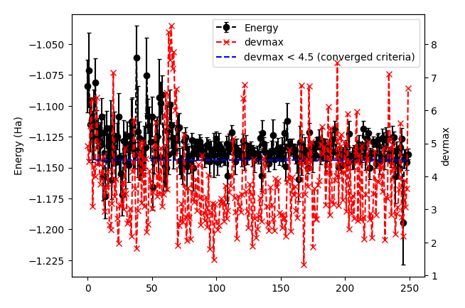
devmax is below the converged criteria of devmax = 4.5, hence we can say the convergence is achieved.

Post-processing performs three important functions:

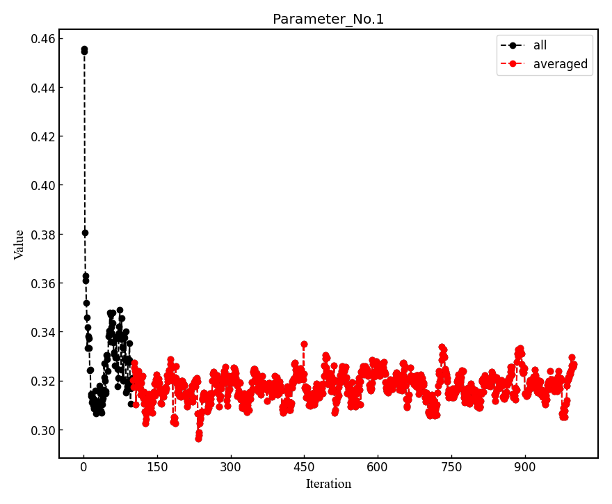
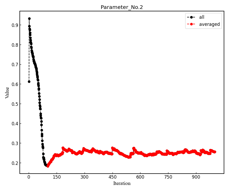
1. The parameters of Jastrow were optimized over \frac{ngen}{nweight} iterations. Post-processing plots all the parameters with respect to iterations which is saved in all_parameters_saved. check png files in parameters_graphs directory (e.g., eog parameters_graphs/Parameter_No*_averaged.png). Here, we show the plots of first two parameters:

   

2. In the second step post-processing averages optimized variational parameters. In our case, this is done over the last several thousands optimisation steps. If you wish to change the number of -optwarmup. The average values of parameters are stored in the file Average_parameters.dat.

3. Finally a dummy vmc calculation is done in ave_temp to write these averaged parameters in fort.10. The final averaged WF is fort.10. The original WF is renamed as fort.10_bak

Warning

For a real run, one should optimize variational parameters much more carefully. We recommend that one consult to an expert or a developer of TurboRVB.

03 VMC (WF=JDFT)

The next step is to run a single-shot VMC calculation, This is done using the vmc module of Turbo-Genius.

First, copy fort.10 from 02optimization to 03VMC and rename it to fort.10

cd ../03vmc/
cp ../02optimization/fort.10 fort.10

Now generate an input file datasvmc.input using:

turbogenius vmc -g -steps 1000 -force

-force (default:False): It allows us to compute VMC forces.

It should look something like the following:

&simulation
    itestr4=2
    ngen=1000
    maxtime=3600
    iopt=1
    disk_io='mpiio'
/

&pseudo
/

&vmc
/

&readio
/

&parameters
    ieskin=1
/

&kpoints
/

Run the VMC calculation:

# on a local machine (serial version)
turborvb-serial.x < datasvmc.input > out_vmc
# on a local machine (parallel version)
mpirun -np XX turborvb-mpi.x < datasvmc.input > out_vmc
# on a cluster machine (PBS)
qsub submit.sh
# on a cluster machine (Slurm)
sbatch submit.sh

After the VMC run finishes, use post-processing to check the total energy:

turbogenius vmc -post -bin 10 -warmup 5

# Note: this corresponds to forces_vmc.sh 10 5 1

Use the following values in this example:

bin length = 10
init bin = 5
pulay = 1 (default)

Chosen values: bin=10, init_bin=5, pulay=1, => equil_steps=50

Postprocessing basically does reblocking using the binning technique. Here again post-processing has two modes: manual and interactive. The reblocked total energy and error are written in the file pip0.d.

% cat pip0.d
Energy =  -1.17274455570072 6.835811355104208E-004

The obtained forces are written in the file forces_vmc.dat.

% cat forces_vmc.dat
Force component 1
Force   = -5.482787285095939E-004  8.061798963778890E-003
1.399428140420830E-003
Der Eloc = -4.043812504378014E-003  7.049753081906847E-003
<OH> =  0.958681484345894       1.543217777712891E-002
<O><H> = -0.956933717457959       1.515228470654634E-002
2*(<OH> - <O><H>) =  3.495533775868420E-003  2.153459465078023E-003

Warning

Force component 1 refers to the sum of the forces of the first line (i.e., 2 1 3 -2 3) in fort.10. The first index is the number of force components and the second and third are the nucleus index and the direction (x:1, y:2, z:3 for a positive nucleus index whereas -x:1, -y:2, -z:3 for a negative nucleus index). Indeed, the forces in the z-direction acting on the first and second hydrogen atoms are -2.74e-4 Ha/Bohr and +2.74e-4 Ha/Bohr, respectively. Not -5.48e-4 Ha/Bohr and +5.48e-4 Ha/Bohr.

04 LRDMC (WF=JDFT)

Lattice regularized diffusion Monte Carlo (LRDMC) is a projection technique that can improve a trial wavefunction obtained by a DFT calculation or a VMC optimization systematically. Indeed, this method filters out the ground state wavefunction from a given trial wavefunction. See the original Casula’s paper, or the review paper in detail.

There is the so-called lattice-space error in LRDMC because the Hamiltonian is regularized by allowing electrons hopping with finite step size alat (Bohr). Therefore, one should extrapolate energies calculated by several lattice spaces (alat) to obtain an unbiased energy (alat \to 0).

Please create each alat folder, and copy an optimized fort.10 from 03vmc to the current alat directory. To generate lrdmc input files for a LRDMC calc.:

cd ../04lrdmc/alat_0.20
cp ../../03vmc/fort.10 .

turbogenius lrdmc -g -etry -1.10 -alat -0.20 -steps 1000

etry Put an obtained DFT or VMC energy. \Gamma in eq.6 of the review paper is set 2 \times etry

alat The lattice space for discretizing the Hamiltonian. If you do a single grid calculation (i.e., alat2=0.0d0), please put a negative value. If you do a double-grid calculation (See the Nakano’s paper), put a positive value and set iesrandoma=.true.. This trick is needed for satisfying the detailed-valance condition.

The input file should look something like:

#datasfn.input
&simulation
    itestr4=-6
    ngen=1000
    iopt=1
    maxtime=1
    disk_io='mpiio'
/

&pseudo
/

&dmclrdmc
    tbra=0.1
    etry=-1.1
    Klrdmc=0.0
    alat=-0.2
    alat2=0.0
    gamma=0.0
    parcutg=1
    typereg=0
    npow=0.0
/

&readio
/

&parameters
/

&kpoints
/

Note

Currently, Turbo-genius automatically sets double grid calculations for all electron systems with Z > 2, and single-grid otherwise. If you want to do something different, please change the input files manually.

alat2 The corser lattice space used in the double-grid calculation. If you put 0.0d0, Turbo does a single grid calculation. If you want to do a double-grid calculation for a compound include Z > 2 element, please comment out alat2 because alat2 is automatically set. See the Nakano’s paper.

Now run the LRDMC calculation:

# on a local machine (serial version)
turborvb-serial.x < datasfn.input > out_fn
# on a local machine (parallel version)
mpirun -np XX turborvb-mpi.x < datasfn.input > out_fn # parallel version
# on a cluster machine (PBS)
qsub submit.sh
# on a cluster machine (Slurm)
sbatch submit.sh

For post-processing use:

turbogenius lrdmc -post -bin 20 -corr 3 -warmup 5
# This corresponds to forcefn.sh 20 3 5 1

Thus, we get E (a=0.20 bohr) = -1.1744(7) Ha.

05 LRDMC (WF=JDFT) Extrapolation.

Warning

For the hydrogen dimer, extrapolation is not needed because the energies are almost constant in the region. Try to plot evsa.gnu with gnuplot later.

If you want to extrapolate energies, please collect all LRDMC energies into evsa.in, # at 04lrdmc directory.

# Preparation of the input files for all alat.
alat_list="0.10 0.40 0.60"
lrdmc_root_dir=`pwd`
for alat in $alat_list
do
cd ../04lrdmc/alat_0.10
cp ../../03vmc/fort.10 .
turbogenius lrdmc -g -etry -1.10 -alat $alat -steps 1000
cd $lrdmc_root_dir
done

# run the jobs
alat_list="0.10 0.40 0.60"
lrdmc_root_dir=`pwd`
for alat in $alat_list
do
    # on a local machine (serial version)
    turborvb-serial.x < datasfn.input > out_fn
    # on a local machine (parallel version)
    mpirun -np XX turborvb-mpi.x < datasfn.input > out_fn # parallel version
    # on a cluster machine (PBS)
    qsub submit.sh
    # on a cluster machine (Slurm)
    sbatch submit.sh
cd $lrdmc_root_dir
done

# Extrapolations of the obtained energies
alat_list="0.10 0.20 0.40 0.60"
lrdmc_root_dir=`pwd`

num=0
echo -n > ${lrdmc_root_dir}/evsa.gnu
for alat in $alat_list
do
    cd alat_${alat}
    num=`expr ${num} + 1`
    echo -n "${alat} " >> ${lrdmc_root_dir}/evsa.gnu
    grep "Energy =" pip0_fn.d  | awk '{print $3, $4}' >> ${lrdmc_root_dir}/evsa.gnu
    cd ${lrdmc_root_dir}
done

sed "1i 1  ${num}  4  1" evsa.gnu > evsa.in  # linear fitting
sed "1i 2  ${num}  4  1" evsa.gnu > evsa.in  # quadratic fitting

funvsa.x < evsa.in > evsa.out

gnuplot
#  p "evsa.gnu" u 1:2:3 with yerr

It performs a curve fitting for energies vs alat. turbo-genius asks for the degree of polynomial to be used for curve fitting. The result of fitting is written to the file evsa.out

For a quartic fitting i.e. E(a)=E(0) + k_{1} \cdots a^2 + k_{2} \cdots a^4, the result is like:

Reduced chi^2  =   8.6591216401279383E-002
Coefficient found
1  -1.1XXXXXXXXXXXXXXXXXXXX        3.2386557773931917E-004  <- E_0
2   9.6921066460640640E-003   1.0580713770253138E-002  <- k_1
3  -4.5430694740357318E-002   6.0957893276622911E-002  <- k_2

For a quadratic fitting i.e. E(a)=E(0) + k_{1} \cdots a^2, the result is like:

Reduced chi^2  =  0.31499156876147028
Coefficient found
1  -1.1XXXXXXXXXXXXXXXXXXXX   2.3072803389120099E-004
2   1.9281569799385230E-003   2.5923005758555885E-003

06 Convert JDFT WF to JAGP one

We have finished all JDFT calculation. The next step is to convert the optimized JDFT ansatz to a JAGPs one.This can be done using convertfort10 module of Turbo-Genius. Basically, we require two fort.10 files: the JDFT one (that we want to convert) and a JAGPs fort10 file which we will use as a template for conversion. The JDFT one should be named as fort.10_in and the JAGPs one should be named as fort.10_out.

Copy fort.10 in 03VMC to 05jdft_to_jagp and rename it as fort.10_in, and copy makefort10.input in 01trial_wavefunction/00makefort10 directory.

cd ../05jdft_to_jagp/
cp ../03vmc/fort.10 .
turbogenius convertwf -to agps

Warning

Here, onebody, twobody, and basis set exponents are read from fort.10_in.

Warning

the original fort.10 is renamed to fort.10_bak

Please check the overlap square in out_conv:

# grep Overlap out_conv
....
Overlap square with no zero  0.9999....

Overlap square should be close to unity, i.e., if the conversion is perfect, this becomes unity.

The converted WF fort.10. This is a JAGPs wavefunction.

The conversion has finished. The obtained JAGPs wavefunction is fort.10.

07 Conversion check

We recommend you should check if the above conversion was successful. This can be checked using the so-called correlated sampling method. Indeed, one can check the difference in energies of WFs using a VMC calculation.

Copy the obtained JAGPs wavefunction fort.10, and the optimized JDFT wavefunction fort.10_in as fort.10_corr:

cd ../06conversion_check/
cp ../05jdft_to_jagp/fort.10 ./fort.10
cp ../05jdft_to_jagp/fort.10_bak ./fort.10_corr

Prepare input files using:

turbogenius correlated-sampling -g -steps 100

For the correlating sampling, we need two input files, for a vmc calculation (i.e., generation of Markov chain) and a correlated sampling itself.

#datasvmc.input
&simulation
    itestr4=2
    ngen=100
    maxtime=3600
    iopt=1
    disk_io='mpiio'
/

&pseudo
/

&vmc
/

&readio
    iread=3
/

&parameters
/

&kpoints
/

and

#readforward.input
&simulation
/

&system
/

&corrfun
    bin_length=1
    initial_bin=1
    correlated_samp=.true.
/

Now run the calculation using:

# on a local machine (serial version)
turborvb-serial.x < datasvmc.input > out_vmc
readforward-serial.x  < datasvmc.input > out_readforward
# on a local machine (parallel version)
mpirun -np XX turborvb-mpi.x < datasvmc.input > out_vmc
mpirun -np XX readforward-mpi.x < datasvmc.input > out_readforward
# on a cluster machine (PBS)
qsub submit.sh
# on a cluster machine (Slurm)
sbatch submit.sh

corrsampling.dat contains the output.

    # corrsampling.dat
Energy (fort10 ref.) = -1.17606202 Ha +- 0.00119647941 Ha
Energy (fort10 corr.) = -1.17606265 Ha +- 0.00119634713 Ha
Energy difference = 6.26299353e-07 Ha +- 2.29651078e-06 Ha
Overlap square = 0.999999977 +- 6.05288029e-08

reweighted difference indicates the difference in energies of the WFs, fort.10 and fort.10_corr. This should be close to zero. Overlap square should be close to unity, i.e., if a conversion is perfect, this becomes unity.

08 Nodal surface optimization (WF=JsAGPs)

In this step, the Jastrow factors and the determinant part are optimized at the VMC level using vmcopt module of Turbo-Genius. The procedure is almost the same as in 02 Jastrow factor optimization (WF=JDFT) First of all, copy the converted wavefunction fort.10

cd ../07optimization/
cp ../05jdft_to_jagp/fort.10 ./

To generate datasmin.input, which is a minimal input file for a VMC-optimization use:

turbogenius vmcopt -g -opt_onebody -opt_twobody -opt_jas_mat -opt_det_mat -optimizer lr -vmcoptsteps 100 -steps 10

The input file should look something like:

&simulation
    itestr4=-4
    ngen=1000
    iopt=1
    maxtime=3600
    disk_io='mpiio'
/

&pseudo
/

&vmc
/

&optimization
    ncg=1
    nweight=10
    nbinr=1
    iboot=0
    tpar=0.35
    parr=0.001
    iesdonebodyoff=.false.
    iesdtwobodyoff=.false.
    twobodyoff=.false.
/

&readio
/

&parameters
    iesd=1
    iesfree=1
    iessw=1
    iesup=0
    iesm=0
/

&kpoints
/

Now run VMC optimization using:

# on a local machine (serial version)
turborvb-serial.x < datasmin.input > out_min
# on a local machine (parallel version)
mpirun -np XX turborvb-mpi.x < datasmin.input > out_min
# on a cluster machine (PBS)
qsub submit.sh
# on a cluster machine (Slurm)
sbatch submit.sh

Now for post-processing use:

turbogenius vmcopt -post -optwarmup 80 -plot

# this corresponds readalles.x

It plots energy with the error bars and devmax wrt optimization steps (vmcopt_Energy_devmax.png).

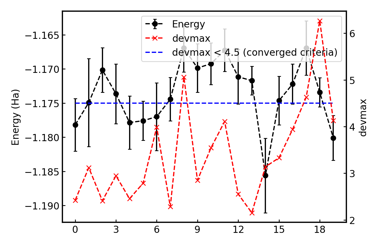
For the hydrogen dimer, the JDFT ansatz is enough accurate, so nothing has gained.

09 VMC (WF=JsAGPs)

The same as in the JDFT case. See 03 VMC (WF=JDFT)

First, copy fort.10 from 02optimization to 08vmc.

cd ../08vmc
cp ../07optimization/fort.10 fort.10

Now generate the input file for vmc datasvmc.input using:

turbogenius vmc -g -steps 1000

Run a VMC calculation by typing:

# on a local machine (serial version)
turborvb-serial.x < datasvmc.input > out_vmc
# on a local machine (parallel version)
mpirun -np XX turborvb-mpi.x < datasvmc.input > out_vmc
# on a cluster machine (PBS)
qsub submit.sh
# on a cluster machine (Slurm)
sbatch submit.sh

After the VMC run finishes, use post-processing to check the total energy:

turbogenius vmc -post -bin 10 -warmup 5
# this corresponds to forcevmc.sh 10 5 1

Use the following values in this example:

bin length = 10
init bin = 5
pulay = 1 (default)

Chosen values: bin=10, init_bin=5, pulay=1, => equil_steps=50

# Note: this corresponds to ``forces_vmc.sh 10 5 1``

Postprocessing basically does reblocking using the binning technique. Here again post-processing has two modes: manual and interactive. The reblocked total energy and error are written to the file energy_error.out. More details are provided in the file pip0.d.

% cat pip0.d
Energy =  -1.17399712181874  4.494314925096871E-004

10 LRDMC (WF=JsAGPs)

The same as in the JDFT case. See 04 LRDMC (WF=JDFT)

cd ../09lrdmc/alat_0.20/
cp ../../08vmc/fort.10 .
turbogenius lrdmc -g -etry -1.10 -alat -0.20 -steps 1000

Now run the LRDMC calculation:

# on a local machine (serial version)
turborvb-serial.x < datasfn.input > out_fn
# on a local machine (parallel version)
mpirun -np XX turborvb-mpi.x < datasfn.input > out_fn # parallel version
# on a cluster machine (PBS)
qsub submit.sh
# on a cluster machine (Slurm)
sbatch submit.sh

For post-processing use:

turbogenius lrdmc -post -bin 20 -corr 3 -warmup 5
# This corresponds to forcefn.sh 20 3 5 1

Thus, we get E (a=0.20 bohr) = -1.1739(4) Ha.

11 Summary

Total energy:

• DFT (PZ-LDA) = -1.1373 Ha

• VMC (JDFT) = -1.1727(7) Ha

• VMC (JAGPs) = -1.1749(4) Ha

• LRDMC (JDFT at a=0.20 bohr) = -1.1744(7) Ha.

• LRDMC (JAGPs at a=0.20 bohr) = -1.1739(4) Ha.

• CCSD(T)=FULL/cc-pVQZ = -1.173793 Ha (Computational Chemistry Comparison and Benchmark DataBase)

12 Preparing a JAGP wavefuction of the H dimer with a shorter bond distance

# preparing a JDFT trial wavefunction
cd 10trial_wavefunction/00makefort10/
turbogenius makefort10 -g -str H2_dimer.xyz -detbasis cc-pVTZ -jasbasis cc-pVDZ -detcutbasis -jascutbasis
turbogenius makefort10 -r
turbogenius makefort10 -post

mv fort.10 fort.10_in
turbogenius convertfort10mol -g -r -post

# run DFT
cd ../01DFT/
cp ../00makefort10/fort.10 ./
turbogenius prep -g -grid 0.2 0.2 0.2 -lbox 10.0 10.0 10.0

# on a local machine (serial version)
prep-serial.x < prep.input > out_prep
# on a local machine (parallel version)
mpirun -np XX prep-mpi.x < prep.input > out_prep
# on a cluster machine (PBS)
qsub submit.sh
# on a cluster machine (Slurm)
sbatch submit.sh

turbogenius prep -post

# conversion
cd ../02jdft_to_jagp/
cp ../01DFT/fort.10_new fort.10
turbogenius convertwf -to agps

13 Nodal surface optimization (WF=JsAGPs)

cd ../../11optimization/
cp ../10trial_wavefunction/02jdft_to_jagp/fort.10 ./
turbogenius vmcopt -g -opt_onebody -opt_twobody -opt_jas_mat -opt_det_mat -optimizer lr -vmcoptsteps 100 -steps 10

# on a local machine (serial version)
turborvb-serial.x < datasmin.input > out_min
# on a local machine (parallel version)
mpirun -np XX turborvb-mpi.x < datasmin.input > out_min
# on a cluster machine (PBS)
qsub submit.sh
# on a cluster machine (Slurm)
sbatch submit.sh

turbogenius vmcopt -post -optwarmup 80 -plot

14 VMC before structural optimization

cd ../12vmc
cp ../11optimization/fort.10 fort.10
turbogenius vmc -g -steps 1000 -force

# on a local machine (serial version)
turborvb-serial.x < datasvmc.input > out_vmc
# on a local machine (parallel version)
mpirun -np XX turborvb-mpi.x < datasvmc.input > out_vmc
# on a cluster machine (PBS)
qsub submit.sh
# on a cluster machine (Slurm)
sbatch submit.sh

turbogenius vmc -post -bin 10 -warmup 5

# check force
%cat forces_vmc.dat
Force component 1
Force   = -0.581448055902718       3.012635556421040E-002
1.943226397097583E-003
Der Eloc = -0.566537913456315       2.996930056497041E-002
<OH> =  0.890900221204126       4.750020105279961E-002
<O><H> = -0.898355292427328       4.681606812429169E-002
2*(<OH> - <O><H>) = -1.491014244640310E-002  3.607617628391403E-003

15 Structural optimization

cd ../13str_optimization
cp ../12vmc/fort.10 ./
turbogenius vmcopt -g -opt_onebody -opt_twobody -opt_jas_mat -opt_det_mat -optimizer lr -vmcoptsteps 100 -steps 10 -opt_structure -strlearn 1.0e-6

# on a local machine (serial version)
turborvb-serial.x < datasmin.input > out_min
# on a local machine (parallel version)
mpirun -np XX turborvb-mpi.x < datasmin.input > out_min
# on a cluster machine (PBS)
qsub submit.sh
# on a cluster machine (Slurm)
sbatch submit.sh

turbogenius vmcopt -post -optwarmup 80 -plot

16 VMC after structural optimization

cd ../14vmc
cp ../13str_optimization/fort.10 fort.10
turbogenius vmc -g -steps 1000 -force

# on a local machine (serial version)
turborvb-serial.x < datasvmc.input > out_vmc
# on a local machine (parallel version)
mpirun -np XX turborvb-mpi.x < datasvmc.input > out_vmc
# on a cluster machine (PBS)
qsub submit.sh
# on a cluster machine (Slurm)
sbatch submit.sh

turbogenius vmc -post -bin 10 -warmup 5

# check force
%cat forces_vmc.dat
Force component 1
Force   =  8.845943906431761E-003  2.073719499651680E-002
1.397654468993750E-003
Der Eloc =  6.856205295579485E-003  2.011093288033853E-002
<OH> =  0.901136545231286       3.656293234452725E-002
<O><H> = -0.900141675925860       3.673121825334205E-002
2*(<OH> - <O><H>) =  1.989738610852276E-003  3.770140210987045E-003