98 Wavefuntion optimization
00 What the VMC optimization does?
From this document, you can learn how to optimize a wavefunction at the VMC level in practice. The most difficult operation in quantum Monte Carlo simulations is to optimize a many-body wavefunction at the VMC level. Here, we describe how to do it in practice. You can also refer to the optimization part (VII. Optimization of WFs) of the review article.
In Variational Monte Carlo, we evaluate the following integral using the Markov-chain monte Carlo method.
E = \cfrac{\int d \vec{R} \cdot \Psi^{*} \left( \vec{R} \right) \cdot \hat{\cal{H}} \Psi \left( \vec{R} \right)}{\int d \vec{R} \cdot \Psi^{*} \left( \vec{R} \right) \Psi \left( \vec{R} \right)}
From the variational principle, the closer to the exact the WF is, the lower the energy becomes. There once we can evaluate the above integral with some variational parameters \vec{\alpha}, we can seek exact solution by minimizing the parameters.
E\left(\vec{\alpha}\right) = \cfrac{\int d \vec{R} \cdot \Psi^{*} \left( \vec{R}, \vec{\alpha} \right) \cdot \hat{\cal{H}} \Psi \left( \vec{R}, \vec{\alpha} \right)}{\int d \vec{R} \cdot \Psi^{*} \left( \vec{R}, \vec{\alpha} \right) \Psi \left( \vec{R}, \vec{\alpha} \right)} \ge E_0
01 Optimization method
There are two major optimization methods are implemented in TurboRVB.
One is the so-called stochastic reconfiguration (SR) method (itestr4 = -9,-5),
and the other one is the so-called linear method (LR) with conjugate gradient (itestr4 = -4,-8). Notice that -9 and -4 do not optimize exponents of the determinant part, while -5 and -8 optimize them.
In general, the LR method works very efficiently and properly when the number of variational parmeters is not so large. For example, less than 1000? If you optimize more than 1000 variational parameters, we recommend the SR method.
02 important hyperparameters
The most important parameters in practice are
tpar: Acceleration parameter (i.e., learning rate.)
parr: Regularization (c.f., LASSO)
tpar
For example, in the stochastic reconfiguration (SR) method, the variational parameters are updated as:
{\alpha _k} \to {\alpha _k} + \Delta \cdot {\left( {{{{\boldsymbol{\mathcal{S'}}}}^{ - 1}}{\mathbf{f}}} \right)_k},
where \Delta is tpar, {\mathbf{f}} is the general force vector, and {\boldsymbol{\mathcal{S'}}} is
the variance-covariance matrix which is stochastically evaluated by means of M configuration samples {\mathbf{x}} = \left\{ {{{\mathbf{x}}_1},{{\mathbf{x}}_2}, \ldots {{\mathbf{x}}_M}} \right\}:
{{\mathcal{S}}_{k,k'}} = \left[ {\frac{1}{M}\sum\limits_{i = 1}^M {\left( {{O_k}\left( {{{\mathbf{x}}_i}} \right) - {{\bar O}_k}} \right) ^ * \left( {{O_{k'}}\left( {{{\mathbf{x}}_i}} \right) - {{\bar O}_{k'}}} \right)} } \right],
where {O_k}\left( {{{\mathbf{x}}_i}} \right) = \frac{{\partial \ln \Psi \left( {{{\mathbf{x}}_i}} \right)}}{{\partial {\alpha _k}}} and {{\bar O}_k} = \frac{1}{M}\sum\limits_{i = 1}^M {{O_k}\left( {{{\mathbf{x}}_i}} \right)}.
parr
The straightforward implementation of the SR method is not stable mainly because the statistical noise sometimes makes the matrix {\boldsymbol{\mathcal{S}}} ill-conditioned, which deteriorates the efficiency of the optimization method. Therefore, in practice, the diagonal elements of the preconditioning matrix {\mathcal{S}} are shifted by a small positive parameter (\varepsilon) as:
{s'_{i,i}} = {s_{i.i}}(1 + \varepsilon ),
where \varepsilon = parr in TurboRVB.
This modification improves the efficiency of the optimization by several orders of magnitude.
03 Order of optimizing variational parameters
The so-called Andrea-Zen’s method empirically works very well for the LR method. Indeed, to avoid local minima in the Jastrow, the developers have experienced that it is important at the beginning to optimize only the one-body Jastrow part. According to this procedure, one should optimize variational parameters in the following order.
Put a reasonable two-body Jastrow parameter (typically ~ 1.0 for -6, -15, -22),
Optimize homogenous and inhomogeneous one-body Jastrows (two-body and three-body are fixed),
Optimize three-body Jastrows (two-body fixed), and
Optimize two-body Jastrow(s) and the determinant part,
wherein
One should set
iesfree=1andiesd=1, and puttwobodyoff=.true.andiesdtwobodyoff=.true.in the¶meterssection,One should remove
iesdtwobodyoff=.true.option, andOne should remove
twobodyoff=.true.andiesdtwobodyoff=.true., and setiessw=1(determinant optimization).
04 Criterium of optimization convergence
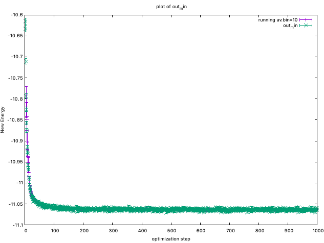
In practice, during an optimization, the code monitors the variational energy (E\left( \boldsymbol{\alpha} \right)) and the maximum value of the signal to noise ratio among all the force components, which is denoted as devmax in the code:
devmax \equiv \max_k \left( {\left| {\frac{{{f_k}}}{{{\sigma _{{f_k}}}}}} \right|} \right)
where {\sigma _{{f_k}}} represents the estimated error bar of a general force {f_k} =- \frac{{\partial E\left( \alpha \right)}}{{\partial {\alpha _k}}} = - \frac{\partial }{{\partial {\alpha _k}}}\frac{{\braket{{\Psi _\alpha }|\hat {\mathcal{H}}|{\Psi _\alpha }}}}{{\braket{{\Psi _\alpha }|{\Psi _\alpha }}}}.
You can plot energies by plot_Energy.sh
You can also plot devmaxs by plot_devmax.sh
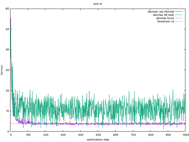
The devepoler has experience that, at least, devmax should be smaller
than 4.0 after optimization. However, the developers also have experienced
that this simple criteria is not sufficient to obtain a converged result.
Instead, the developers recently checked if the two-body Jastrow and the inhomogeneous one-body Jastrows are also converged.
This seems an empirically good criterium of optimization convergence,
though it is still under debate.
05 Hyperparameters in the optimization methods
There are several hyperparameters in the optimization method. Although a proper choice for some hyperparameters are still under debate, we show a tentative guidline.
05-01 nweight
nweight is the number of Monte Carlo sampling per optimization step.
For the LR method, the number of samplings in VMC should be much larger than the number of variational parameters, i.e., nweight \times Number of (mpi) tasks > 5 \sim 10 \times p, where p is the number of variational parameters.
For the SR method, nweight \times Number of (mpi) tasks can be set even or smaller than p as long as parr is set sufficiently large.
05-02 tpar
tpar is an acceleration hyperparameter in optimization, corresponding to Delta in Eq.131 and that in Eq.139 of the review paper for the LR and SR methods, respectively. In the machine learning community, tpar is also called learning rate.
For the LR method, tpar = 0.35 usually works well.
For the SR method, one should set tpar much smaller, typically 1.0d-4.
adjust_tpar is a useful option recently introduced by Andrea Tirelli, to find an optimal tpar. Indeed, if adjust_tpar is set true, tpar gradually increases as optimization iteration goes on after 100 equilibrium iterations.
beta_learning is also a useful option to realize a stable optimization. beta_learning = 0.90 is a good starting point?
05-03 parr
parr is a regularization parameter which is added to the diagonal elements of a preconditioning matrix S, in Eq.128 of the review paper.
In the LR method, XXX
KN is now working…
05-04 ncg
This works only for the LR method.
KN is now working…
05-05 npbra and parcurpar
This works only for the LR method.
KN is now working…