Wave functions

Both the accuracy and the computational efficiency of QMC approaches crucially depend on the WF ansatz. The optimal ansatz is typically a tradeoff between accuracy and efficiency. On the one side, a very accurate ansatz can be involved and cumbersome, having many parameters and being expensive to evaluate. On the other hand, an efficient ansatz is described only by the most relevant parameters and can be quickly and easily evaluated. In particular, in the previous sections, we have seen that QMC algorithms, both at the variational and fixed-node level, imply several calculations of the local energy \(e_L(\mathbf{x})\) and the ratio \(\Psi(\mathbf{x})/\Psi(\mathbf{x}')\) for different electronic configurations \(\mathbf{x}\) and \(\mathbf{x}'\). The computational cost of these operations determines the overall efficiency of QMC and its scaling with systems size.

jQMC employs a many-body WF ansatz \(\Psi\) which can be written as the product of two terms:

\[ \Psi = \Phi _\text{AS} \times \exp J \,, \]

where the term \(\exp J\), conventionally dubbed Jastrow factor, is symmetric under electron exchange, and the term \(\Phi _\text{AS}\), also referred to as the determinant part of the WF, is antisymmetric. The resulting WF \(\Psi\) is antisymmetric, thus fermionic.

In the majority of QMC applications, the chosen \(\Phi _\text{AS}\) is a single Slater determinant (SD) \(\Phi _\text{SD}\), {\it i.e.}, an antisymmetrized product of single-electron WFs. % (\({\cal A}\{\psi_1(1) \psi_2(2) \ldots \psi_N(N) \}\)). Clearly, SD alone does not include any correlation other than the exchange. However, when a Jastrow factor, explicitly depending on the inter-electronic distances, is applied to \(\Phi _\text{SD}\) the resulting ansatz \(\Psi_\text{JSD} = \Phi _\text{SD} * \exp J\) often provides over 70% of the correlation energy[1] at the variational level. Thus, the Jastrow factor proves very effective in describing the correlation, employing only a relatively small number of parameters, and therefore providing a very efficient way to improve the ansatz.[2] A Jastrow correlated SD (JSD) function yields a computational cost for QMC simulations – both VMC and FN – about \(\propto N^3\), namely the same scaling of most DFT codes. Therefore, although QMC has a much larger prefactor, it represents an approach much cheaper than traditional quantum chemistry ones, at least for large enough systems.

While the JSD ansatz is quite satisfactory in several applications, there are situations where very high accuracy is required, and a more advanced ansatz is necessary. The route to improve JSD is not unique, and different approaches have been attempted within the QMC community. First, it should be mentioned that improving the Jastrow factors is not an effective approach to achieve higher accuracy at the FN level, as the Jastrow is positive and cannot change the nodal surface.

The strategy employed in jQMC is inspired by the pioneering work of TurboRVB and is that the route toward an improved ansatz should not compromise the efficiency and good scaling of QMC. For this reason, neither backflow nor explicit multideterminant expansions are implemented in the code. Within the jQMC project, the main goal is instead to consider an ansatz that can be implicitly equivalent to a multideterminant expansion, but remains in practice as efficient as a single determinant.

jQMC currently offers three alternatives for the choice of \(\Phi_\text{AS}\), which correspond to

1. the Antisymmetrized Geminal Power (AGP),

2. the AGP with constrained number of molecular orbitals (AGPn), and

3. the single Slater determinant.

In QMC, the WFs are always meant to include the Jastrow factor, which proves fundamental to improve the properties of the overall WF. For instance, AGP carries more correlation than SD. However, it is not size-consistent unless it is multiplied by a Jastrow factor. Thus, a fundamental step to take advantage of the WF ansatz is the possibility to perform reliable optimizations of the parameters. Optimization will be discussed in section Variational Monte Carlo (VMC). In this section, we will describe the functional form of the Jastrow factor implemented in jQMC (sec. Jastrow factor (J)), the AGP (sec. Antisymmetrized Geminal Power (AGP)), the AGPn (sec. AGP with constrained number of molecular orbital (AGPn)), the SD (sec. Single Slater determinant (SD)), the summary of the anstaz (sec. Summary: Many-body wavefunction), and the basis set and atomic orbitals used in the Jastrow and the AS parts (sec. Atomic orbitals (AOs) and Basis sets).

Jastrow factor (J)

The Jastrow factor (\(\exp J\)) plays an important role in improving the correlation of the WF and in fulfilling Kato’s cusp condition [T. Kato, Commun. Pure Appl. Math. 10, 151 (1957)]. jQMC implements the Jastrow term composed of one-body, two-body, and three/four-body factors (\(J = {J_1}+{J_2}+{J_{3/4}}\)). The one-body and two-body factors are used to fulfill the electron-ion and electron-electron cusp conditions, respectively, and the three/four-body factors are employed to consider a systematic expansion, in principle converging to the most general independent electron pairs contribution. The one-body Jastrow factor \(J_1\) is the sum of two parts, the homogeneous part (enforcing the electron-ion cusp condition):

(1)\[ J_1^{\rm h} \left( \mathbf{r}_1,\ldots,\mathbf{r}_N \right) = \sum_{i=1}^{N_{\rm{e}}} \sum_{\alpha=1}^{N_\text{a}} \left( { { - {{\left( {2{Z_{\alpha}}} \right)}^{3/4}}u\left( {(2{Z_{\alpha}})^{1/4}\left| {{\mathbf{r}_i} - {{\mathbf{R}}_{\alpha}}} \right|} \right)} } \right), \]

and the corresponding inhomogeneous part:

(2)\[ {J_1^{\rm inh}}\left( {{{\mathbf{r}}_1}, \ldots, {{\mathbf{r}}_N}} \right) = \sum_{i=1}^{N_{\rm{e}}} \sum_{\alpha=1}^{N_\text{a}} \left( {\sum\limits_{l} {M_{\alpha,l} \chi_{\alpha,l}\left( {{{\mathbf{r}}_i}} \right)} } \right) , \]

where \({{{\mathbf{r}}_i}}\) are the electron positions, \({{{\mathbf{R}}_{\alpha}}}\) are the atomic positions with corresponding atomic number \(Z_{\alpha}\), \(l\) runs over atomic orbitals \(\chi _{\alpha,l}\) ({\it e.g.}, GTO) centered on the atom \(a\), \(\{ M_{\alpha,l} \}\) are variational parameters, and \({u_a\left( \mathbf{r} \right)}\) is a simple bounded function. In jQMC, the most common choice for \(u\) is:

(3)\[ u\left( r \right) = \frac{ 1 }{2 b_{\text{ei}}} \left( {1 - {e^{ - r b_{\text{ei}}}}} \right) \,, \]

depending on a single variational parameter \( b_{\text{ei}}\).

The two-body Jastrow factor is defined as:

(4)\[ {J_2}\left( {{{\mathbf{r}}_1}, \ldots, {{\mathbf{r}}_N}} \right) = {\sum\limits_{i < j} {{v_{{\sigma _i},{\sigma _j}}}\left( {\left| {{{\mathbf{r}}_i} - {{\mathbf{r}}_j}} \right|} \right)} }, \]

where \(v_{{\sigma _i},{\sigma _j}}\) is another simple bounded function. There are several possible choices for \(v_{{\sigma _i},{\sigma _j}}\) implemented in jQMC is the following spin-independent form:

(5)\[\begin{split} {v_{{\sigma _i},{\sigma _j}}}\left( {{r_{i,j}}} \right) = \begin{cases} \cfrac{{{r_{i,j}}}}{2} \cdot {\left( {1 + b_{\rm{ee}} \cdot {{r_{i,j}}}} \right)^{ - 1}} & ({\sigma _i} = {\sigma _j}) \\ \cfrac{{{r_{i,j}}}}{2} \cdot {\left( {1 + b_{\rm{ee}} \cdot {{r_{i,j}}}} \right)^{ - 1}} & ({\sigma _i} \neq {\sigma _j}) \end{cases} \end{split}\]

where \({r_{i,j}} = \left| {{{\mathbf{r}}_i} - {{\mathbf{r}}_j}} \right|\), and \(b_{\rm{ee}}\) is the common variational parameter.

The three/four-body Jastrow factor reads:

(6)\[ J_{3/4}\left( {{{\mathbf{r}}_1}, \ldots, {{\mathbf{r}}_N}} \right) = \sum_{i < j} \left( \sum_{l} \sum_{l'} M_{l,l'} \chi _{l}( \mathbf{r}_i ) \chi _{l'}( \mathbf{r}_j ) \right), \]

where the indices \(l\) and \(l'\) indicate different orbitals and \(\{ M_{l,l'} \}\) are variational parameters.

To exploit JAX accelerations, one should implement computations with the numpy style (i.e., matrix-vector and/or matrix-matrix operations). The inhomogeneous one-body (\(J_{\rm inh}\)) and three/four-body Jastrow (\(J_{3/4}\)) factors can be implemented by matrix-vector and matrix-matrix operations. The one-body term \({J_1^{inh}}\left(\ldots, {{\mathbf{r}}_i}, \ldots \right)\) is computed as:

\[\begin{split} \begin{aligned} {J_1^{\rm inh}}\left(\ldots, {{\mathbf{r}}_i}, \ldots \right) &= \sum_{u=1}^{N_e^{\uparrow}} \sum_{l=1}^{L} \left( { {M_{l} \chi_{l} ( \vec{r}_u^{\uparrow})} } \right) + \sum_{d=1}^{N_e^{\downarrow}} \sum_{l=1}^{L} \left( { {M_{l} \chi_{l} ( \vec{r}_d^{\downarrow})} } \right) \\ &= M X^{\uparrow} \vec{e}^{N_e^{\uparrow}} + M X^{\downarrow} \vec{e}^{N_e^{\downarrow}}, \end{aligned} \end{split}\]

where \(\vec{e}^{N_e^{\uparrow}}\) and \(\vec{e}^{N_e^{\downarrow}}\) are \((N_e^{\uparrow}, 1)\) and \((N_e^{\downarrow}, 1)\) unit column vectors, \(X^{\uparrow}_{l,u} \equiv \chi _{l}( \vec{r}_{u}^{\uparrow} )\) is \((L, N_e^{\uparrow})\) matrix, \(X^{\downarrow}_{l',d} \equiv \chi _{l'}( \vec{r}_{d}^{\downarrow} )\) is \((L, N_e^{\downarrow})\) matrix, and \(M\) is \((L, L)\) matrix.

The three-body term \(J_{3/4}\left( {{{\mathbf{r}}_1}, \ldots, {{\mathbf{r}}_N}} \right)\) is computed as:

\[\begin{split} \begin{aligned} J_{3/4}\left( {{{\mathbf{r}}_1}, \ldots, {{\mathbf{r}}_N}} \right) &= \sum_{u' > u}^{N_e^{\uparrow}, N_e^{\uparrow}} \left( \sum_{l,l'}^{L, L} \chi _{l}( \vec{r}_{u}^{\uparrow} ) M_{l,l'} \chi _{l'}( \vec{r}_{u'}^{\uparrow} ) \right) + \sum_{d' > d}^{N_e^{\downarrow}, N_e^{\downarrow}} \left( \sum_{l,l'}^{L, L} \chi _{l}( \vec{r}_{d}^{\downarrow} ) M_{l,l'} \chi _{l'}( \vec{r}_{d'}^{\downarrow} ) \right) + \sum_{u,d}^{N_e^{\uparrow}, N_e^{\downarrow}} \left( \sum_{l,l'}^{L, L} \chi _{l}( \vec{r}_{u}^{\uparrow} ) M_{l,l'} \chi _{l'}( \vec{r}_{d}^{\downarrow} ) \right) \\ &= \operatorname{tr} \left( (X^{\uparrow})^T M X^{\uparrow} K^{\uparrow} \right) + \operatorname{tr} \left( (X^{\downarrow})^T M X^{\downarrow} K^{\downarrow} \right) + (\vec{e}^{N_e^{\uparrow}})^T (X^{\uparrow})^T M X^{\downarrow} \vec{e}^{N_e^{\downarrow}}, \end{aligned} \end{split}\]

where \(K^{\uparrow}\) and \(K^{\downarrow}\) are \((N_e^{\uparrow}, N_e^{\uparrow})\) and \((N_e^{\downarrow}, N_e^{\downarrow})\) matrices, reading:

\[\begin{split} \kappa_{i,j} = \begin{cases} 1 & (i > j) \\ 0 &(i \le j) \end{cases}. \end{split}\]

Neural Network Jastrow Factor

We augment the Jastrow factor with a neural-network term \(J_{\text{NN}}\) using a PauliNet-inspired GNN [Hermann et al., Nat. Chem. 12, 891 (2020)]. Inputs are electron coordinates \(\{\mathbf{r}_i\}_{i=1}^{N_e}\) with spins \(s_i \in \{\uparrow,\downarrow\}\), nuclear coordinates \(\{\mathbf{R}_I\}_{I=1}^{N_n}\), and atomic numbers \(\{Z_I\}\). The architecture is translationally and rotationally invariant and symmetric under exchange of electrons within each spin channel; fermionic antisymmetry is carried by the Slater/Geminal part. Variational parameters in this VMC setting are all trainable weights and biases of the neural networks described below, including spin embeddings, nuclear (species) embeddings, the message/receiver networks, and the readout network.

Input Features

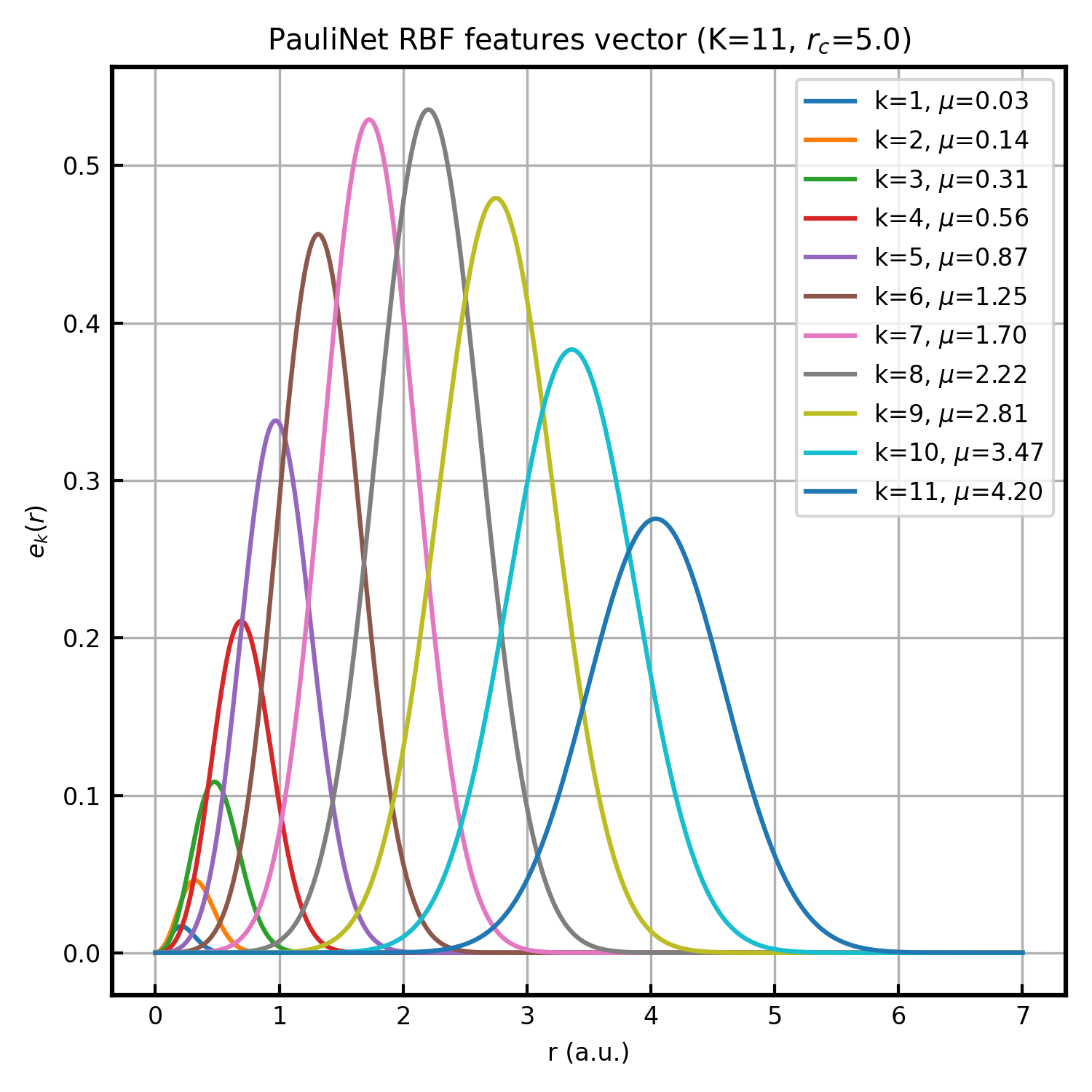
Geometry is encoded solely by scalar distances: electron–electron \(r_{ij}=|\mathbf{r}_i-\mathbf{r}_j|\) and electron–nucleus \(r_{iI}=|\mathbf{r}_i-\mathbf{R}_I|\) (nucleus–nucleus distances are constant under the Born–Oppenheimer approximation). Each distance is expanded into PhysNet-style radial basis functions (RBFs) parametrized in the PauliNet paper:

\[ e_k(r) = r^2 \exp\!\left[-r - \frac{(r-\mu_k)^2}{\sigma_k^2}\right], \]

where \(\mu_k\) and \(\sigma_k\) are hyperparameters determined by the grid points \(q_k\). The prefactor \(r^2\) makes the feature and its derivative vanish at \(r=0\), so \(J_{\text{NN}}\) preserves the electron–nucleus cusp enforced by analytic terms. The number of basis functions \(K\) is set by num_rbf, and the parameter cutoff (\(r_c\)) determines the distribution range of the basis function centers (user inputs). The parameters are defined as \(\mu_k = r_c q_k^2, \quad \sigma_k = \frac{1}{7}(1 + r_c q_k)\), where \(\{q_k\}_{k=1}^K\) are \(K\) points evenly spaced in the interval \((0, 1)\).

Interaction Layers

Each electron carries a latent feature \(\mathbf{x}_i^{(l)} \in \mathbb{R}^F\) at layer \(l\), where the latent width \(F\) is set by hidden_dim (user input). Initialization (\(l=0\)) is the sum of a spin embedding (depends on \(s_i\)) and a one-body nuclear context. The total number of message-passing layers \(L\) is set by num_layers (user input). For \(l=0,\dots,L-1\), we update \(\mathbf{x}_i^{(l)}\) by aggregating channel-specific neighborhoods: same-spin \(\mathcal{N}_{\parallel}(i)=\{j\neq i \mid s_j=s_i\}\), opposite-spin \(\mathcal{N}_{\perp}(i)=\{j \mid s_j\neq s_i\}\), and nuclei \(\mathcal{N}_{n}(i)=\{I \mid 1\le I\le N_n\}\). The update is

\[ \mathbf{x}_i^{(l+1)} = \mathbf{x}_i^{(l)} + \sum_{\nu \in \{\parallel,\perp,n\}} \mathcal{F}_{\text{recv}}^{(\nu)} \!\left( \sum_{j \in \mathcal{N}_\nu(i)} \mathcal{G}^{(\nu)}(\mathbf{e}(r_{ij})) \odot \mathbf{h}_j^{(\nu)} \right), \]

where \(\mathbf{e}(r_{ij})\) is the RBF vector for the relevant distance (\(r_{ij}\) for electrons, \(r_{iI}\) for nuclei). For electron channels (\(\nu\in\{\parallel,\perp\}\)), the sender feature is \(\mathbf{h}_j^{(\nu)}=\mathbf{x}_j^{(l)}\); for the nuclear channel (\(\nu=n\)), \(\mathbf{h}_I^{(n)}\) is a learnable species embedding determined by \(Z_I\) (layer-independent). Both \(\mathcal{G}^{(\nu)}:\mathbb{R}^K \to \mathbb{R}^F\) and \(\mathcal{F}_{\text{recv}}^{(\nu)}:\mathbb{R}^F \to \mathbb{R}^F\) are standard fully-connected neural networks (two linear layers with SiLU activation). The Hadamard product \(\odot\) applies the interaction filter to the sender feature, and the residual addition stabilizes training. All weights/biases in these networks, including embeddings, are variational parameters.

Global Readout

After \(L\) layers, permutation invariance is enforced by summing the outputs of a channel-wise readout network:

\[ J_{\text{NN}} = \sum_{i=1}^{N_e} \text{NN}_{\text{readout}}(\mathbf{x}_i^{(L)}). \]

The readout uses a fully-connected neural network (two linear layers with SiLU, output dimension 1). The summation over all electrons ensures the symmetry required for the Jastrow factor. The readout weights and biases are also variational parameters optimized within VMC.

Antisymmetrized Geminal Power (AGP)

jQMC implementes Antisymmetrized Geminal Power (AGP) anstaz for the antisymmetric part, which was applied to the {\it ab initio} calculation by M. Casula and S. Sorella [M. Casula and S. Sorella, J. Chem. Phys. 119, 6500 (2003)] for the first time in 2003; then it has been also implemented in other QMC codes. For simplicity, let us first consider a system with an even number \(N\) of electrons. The WF, written in terms of pairing functions, is:

(7)\[ \Phi_\text{AS} (\mathbf{1},\ldots,\mathbf{N}) = {\cal A} \left\{ g(\mathbf{1},\mathbf{2}) g(\mathbf{3},\mathbf{4}) \ldots g(\mathbf{N-1},\mathbf{N}) \right\} \]

where \({\cal A}\) is the antisymmetrization operator:

\[ {\cal A} \equiv {1\over N!} \sum_{P\in S_N} \epsilon_P \hat P, \]

\(S_N\) the permutation group of \(N\) elements, \(\hat P\) the operator corresponding to the generic permutation \(P\), and \(\epsilon_P\) its sign. We denote with the generic bolded index \(\mathbf{i}\) both the space \({\bf r}_i\) coordinates and the spin values \(\sigma_i\):

\[ \mathbf{i} \leftrightarrow ({\bf r}_i, \sigma_i) \]

corresponding to the \(i^{th}\) electron.

Let us define \(G\) the \(N\times N\) matrix with elements \(G_{i,j} = g(\mathbf{i},\mathbf{j})\). Notice that

\[ g(\mathbf{i},\mathbf{j}) = -g(\mathbf{j},\mathbf{i}) \; (\text{and} \; G_{i,j} = -G_{j,i}), \]

as a consequence of the statistics of fermionic particles, thus \(G\) is skew-symmetric ({\it i.e.}, \(G^T = -G\), being \(^T\) the transpose operator).

We parameterize the pairing function \(g\) with generalized spin-dependent orbitals \(\phi(r, \sigma) \equiv \psi(r)\chi(\sigma)\), where \(\psi\) is its spatial part and \(\chi\) is the spin function. For 2\(L\) orbitals,

\[ (\psi_1^{\alpha}(r)\alpha_1(\sigma) \cdots \psi_L^{\alpha}(r)\alpha_L(\sigma) \cdots \psi_1^{\beta}(r)\beta_1(\sigma) \cdots \psi_L^{\beta}(r)\beta_L(\sigma) ), \]

the pairing function is parameterized as:

\[ g(i, j) = \sum_{\mu,\nu} A_{\mu,\nu} \phi_{\mu}(r_i, \sigma_i) \phi_{\nu}(r_j, \sigma_j) \equiv \sum_{\mu,\nu} A_{\mu,\nu} \psi_{\mu}(r_i)\psi_{\nu}(r_j)\chi_{\mu}(\sigma_i)\chi_{\nu}(\sigma_j) \]

where \(A_{\mu,\nu}\) is a \((2L,2L)\) skew-symmetric matrix as a consequence of \(g(i,j) = - g(j,i)\).

jQMC currently considers only the pairing functions with opposite spins, thus, the antisymmetrization operator corresponds to the determinant of the up-down or down-up pairing matrix \(G\), i.e.,

\[ \Phi(1 \cdots N) = \det(G_{u,d}) = - \det(G_{d,n}) \]

We denote block matrices \(\Lambda^{\uparrow, \downarrow}_{l,l'} \equiv A_{u,d}\) and \(\Lambda^{\downarrow, \uparrow}_{l,l'} \equiv A_{d,n}\), where \(l\) and \(l'\) run over from 1 to \(L\). Since \(A\) is skew-symmetric, \(\Lambda^{\uparrow, \downarrow}_{l,l'} = - \Lambda^{\downarrow, \uparrow}_{l',l}\). Indeed, one can consider up and down pairs without loss of generality. Say, we can omit the spin-dependent part in practice, and for a spatial generic pairing function \(F_{i,j} \equiv f(r_i^{\uparrow}, r_j^{\downarrow})\) we have

(8)\[ f\left( {{{\mathbf{r}}_i^{\uparrow}},{{\mathbf{r}}_j}^{\downarrow}} \right) = \sum\limits_{l,l'} {\Lambda_{l,l'}^{\uparrow, \downarrow} {\psi_{l}^{\uparrow}}\left( {{{\mathbf{r}}_i^{\uparrow}}} \right){\psi _{l'}^{\downarrow}}\left( {{{\mathbf{r}}_j^{\downarrow}}} \right)}, \]

and

\[ \Phi(1 \cdots N) = \det(G_{u,d}) = \det(F). \]

Hereafter, we think about cases with spin-independent orbitals \(\psi^{\alpha} = \psi^{\beta}\). In such a case, the generalized pairing function for opposite spins is parametrized as

\[\begin{split} \begin{aligned} g(i, j) &= \sum_{l,l'} \Lambda_{l,l'}^{\uparrow, \downarrow} \psi_{l}(r_i)\psi_{l'}(r_j)\alpha(\sigma_i)\beta(\sigma_j) + \sum_{l,l'} \Lambda_{l,l'}^{\downarrow, \uparrow} \psi_{l}(r_i)\psi_{l'}(r_j)\beta(\sigma_i)\alpha(\sigma_j) \\ &= \sum_{l,l'} \Lambda_{l,l'}^{\uparrow, \downarrow} \psi_{l}(r_i)\psi_{l'}(r_j)\alpha(\sigma_i)\beta(\sigma_j) - \sum_{l,l'} \Lambda_{l',l}^{\uparrow, \downarrow} \psi_{l}(r_i)\psi_{l'}(r_j)\beta(\sigma_i)\alpha(\sigma_j) \\ \end{aligned} \end{split}\]

If \(\Lambda_{l,l'}\) is symmetric, \( \Lambda_{l',l}^{\uparrow, \downarrow} = \Lambda_{l,l'}^{\uparrow, \downarrow} \equiv \Lambda_{l,l'}^S \), leading to:

\[\begin{split} \begin{aligned} g(i, j) &= \sum_{l,l'} \Lambda_{l,l'}^{\uparrow, \downarrow} \psi_{l}(r_i)\psi_{l'}(r_j)(\alpha(\sigma_i)\beta(\sigma_j) - \beta(\sigma_i)\alpha(\sigma_j)) \\ &= \sum_{l,l'} \Lambda_{l,l'}^{S} \psi_{l}(r_i)\psi_{l'}(r_j)(\alpha(\sigma_i)\beta(\sigma_j) - \beta(\sigma_i)\alpha(\sigma_j)) \\ &\equiv f_{S}({\bf r}_i,{\bf r}_j) ({ {\left| \uparrow \downarrow \right\rangle - \left| \downarrow \uparrow \right\rangle}}), \end{aligned} \end{split}\]

which is dubbed as AGP with spin-singlet pairs (AGPs).

If \(\Lambda_{l,l'}\) is skew-symmetric, \( \Lambda_{l',l}^{\uparrow, \downarrow} = - \Lambda_{l,l'}^{\uparrow, \downarrow} \equiv \Lambda_{l,l'}^A \), leading to:

\[\begin{split} \begin{aligned} g(i, j) &= \sum_{l,l'} \Lambda_{l,l'}^{\uparrow, \downarrow} \psi_{l}(r_i)\psi_{l'}(r_j)(\alpha(\sigma_i)\beta(\sigma_j) + \beta(\sigma_i)\alpha(\sigma_j)) \\ &= \sum_{l,l'} \Lambda_{l,l'}^{A} \psi_{l}(r_i)\psi_{l'}(r_j)(\alpha(\sigma_i)\beta(\sigma_j) + \beta(\sigma_i)\alpha(\sigma_j)) \\ &\equiv f_{T}({\bf r}_i,{\bf r}_j) ({ {\left| \uparrow \downarrow \right\rangle + \left| \downarrow \uparrow \right\rangle}}), \end{aligned} \end{split}\]

which is dubbed as AGP with spin-singlet pairs with triplet correlations (AGPt).

Even if \(\Lambda^{l,l'}\) is neither symmetric nor skew-symmetric, the components corresponding to AGPs and AGPu can be uniquely recovered because any square matrix can be uniquely decomposed into a sum of a symmetric and a skew-symmetric matrix [G. Strang, Linear Algebra and Its Applications (2009)]. In such a case, the resultant pairing function is the combination of AGPs and AGPt.

In this sense, if basis is spin-dependent, the sptial and spin parts cannot be separated and the spin-singlet pairings are no longer eigenstates, introducing a spin-contaminated pairing function, dubbed as AGPc.

In the above formalism, AGPs, AGPt, AGPs+AGPt, AGPc are separately defined. However, in the actual implementation, we define only one matrix \(\Lambda_{l,m}\) and compute the spatial part of the pairing function as:

\[ f(\mathbf{r}_i, \mathbf{r}_j) = \sum_{l,m} \Lambda_{l,l'}^{\uparrow, \downarrow} \, \phi_l^{\uparrow}(\mathbf{r}_i)\, \phi^{\downarrow}_{l'}(\mathbf{r}_j). \]

Accordingly, in the implementation, the distinction between AGPs, AGPt, AGPs + AGPt, and AGPc is determined by the spatial part of the basis and the symmetry of the matrix \(\Lambda^{\uparrow, \downarrow}\)-whether it is symmetric, skew-symmetric, or neither-allowing all cases to be handled within a unified framework.

The AGP ansatz can be generalized to describe polarized systems, {\it i.e.}, systems where the number \(N_u\) of electrons of spin up is different from the number \(N_d\) of electrons with spin down. With no loss of generality, we can assume that \(N_u>N_d\), thus the system is constituted by a number \(p=N_d\) of electron pairs and a number \(k=N_u-N_d\) of unpaired electrons (clearly, \(N=N_u+N_d=2p+k\)). For spin-polarized systems with unpaired orbitals, we can add \(k\) fictitious entries to \(g(\mathbf{i},\mathbf{j})\), such that \(g(\mathbf{i},\mathbf{N+l})=-g(\mathbf{N+l},\mathbf{i}) = \phi_l(\mathbf{i})\) for \(l=1,\ldots,k\) and \(i=1,\ldots,N_u\).

Thus, we need to evaluate:

(9)\[ \Phi_\text{AGP} = \det(\tilde G) \,. \]

with the \(N_u\times N_u\) matrix \(\tilde G = \left[\begin{array}{c|c} G_{ud} & \Phi \end{array}\right]\), where the \(N_u\times N_d\) matrix \(G_{ud}\) describes the pairing between the \(N_u\) spin up electrons and the \(N_d\) spin down electrons, and the \(N_u\times k\) matrix \(\Phi\) describes the \(k\) unpaired orbitals.

Here, we describe a practical implementation of the pairing function calculation. As written above, to exploit JAX accelerations, one should implement computations with the numpy style (i.e., matrix-vector and/or matrix-matrix operations). Suppose one evaluates the value of a many-body WF at \(\vec{x}^{\uparrow} = (\vec{r}_1^{\uparrow}, \cdots, \vec{r}_i^{\uparrow}, \cdots, \vec{r}^{\uparrow}_{N_{e}^{\uparrow}})\) and \(\vec{x}^{\downarrow} = (\vec{r}_1^{\downarrow}, \cdots, \vec{r}_j^{\downarrow}, \cdots, \vec{r}^{\downarrow}_{N_{e}^{\downarrow}})\).

The basis set expanding AGP pairing function is arbitary; thus, jQMC support the expansion with both atomic and molecular orbitals. Both AGP with Molecular Orbitals and AGP with Atomic Orbitals can be treated in the same way in practice.

For the paired parts with AOs, we can prepare for a lambda matrix \(\Lambda^{\uparrow, \downarrow}\), i.e., \(\lambda_{l,m}^{\uparrow, \downarrow}\), whose dimension is (\(M_{ao}, M_{ao}\)) and, atomic or molecular orbitals matrix, \(\Psi_{l,i}^{\uparrow} = \psi^{\uparrow}_l(\vec{r}_i^{\uparrow})\), \(\Psi_{m,j}^{\downarrow} = \psi^{\downarrow}_m(\vec{r}_j^{\downarrow})\), whose dimensions are \((M_{ao}, N_{e}^{\uparrow})\) and \((M_{ao}, N_{e}^{\downarrow})\). Here, we assume that the number of AOs is the same for up and down electrons such that the geminal matrix \(\Lambda^{\uparrow, \downarrow}\) is square. Then, the pairing geminal matrix is \(F(\vec{x}^{\uparrow}, \vec{x}^{\downarrow}) = (\Psi^{\uparrow})^T \Lambda^{\uparrow, \downarrow} \Psi^{\downarrow}\), where \(F_{i,j} = \sum_{l,m} \Psi_{i,l}^{\uparrow} \lambda_{l,m}^{\uparrow, \downarrow} \Psi_{m,j}^{\downarrow}\). The dimension of \(F\) matrix is \((N_{e}^{\uparrow}, N_{e}^{\downarrow})\). For the unpaired part, a lambda matrix \(\Lambda^{\uparrow}\), whose dimension is (\(M_{ao}, N_{e}^{\uparrow} - N_{e}^{\downarrow}\)), and \(\Psi_{l,i}^{\uparrow} = \psi^{\uparrow}_l(\vec{r}_i^{\uparrow})\), whose dimensions are \((M_{ao}, N_{e}^{\uparrow})\). The unpaired part can be computed as \(F(\vec{x}^{\uparrow}) = (\Psi^{\uparrow})^T \Lambda^{\uparrow}\), where \(F_{i,k} = \sum_{l} \Psi_{i,l}^{\uparrow} \lambda_{l,k}^{\uparrow}\), whose dimension is \((N_{e}^{\uparrow}, N_{e}^{\uparrow} - N_{e}^{\downarrow})\).

Then, the determinant part is computed as \(\det (\tilde{F}(\vec{x}^{\uparrow}, \vec{x}^{\downarrow}))\), where \(\tilde{F}(\vec{x}^{\uparrow}, \vec{x}^{\downarrow})\) is the concatenated matrix, whose dimension is \((N_{e}^{\uparrow}, N_{e}^{\uparrow})\), i.e., \(\tilde{F}(\vec{x}^{\uparrow}, \vec{x}^{\downarrow}) = [(\Psi^{\uparrow})^T \Lambda^{\uparrow, \downarrow} \Psi^{\downarrow} | (\Psi^{\uparrow})^T \Lambda^{\uparrow} ]\). From the practical view point, we can set the input variational parameters as a concatenated matrix \(\tilde{\Lambda} \equiv [\Lambda^{\uparrow, \downarrow} | \Lambda^{\uparrow}]\), whose dimension is \((M_{ao}, M_{ao} + N_{e}^{\uparrow} - N_{e}^{\downarrow})\).

MO cases are the same as the AO cases by setting \(\Psi_{l,i}^{\uparrow} = \phi_l^{\uparrow}(\vec{r}_i^{\uparrow})\), \(\Psi_{m,j}^{\downarrow} = \phi_m^{\downarrow}(\vec{r}_j^{\downarrow})\), whose dimensions are \((M_{mo}, N_{e}^{\uparrow})\) and \((M_{mo}, N_{e}^{\downarrow})\). The MOs can be different for up and down electrons in the case of UHF/UKS calculations.

Since MOs and AOs are connected via the following relation:

\[\begin{split} \begin{gathered} \Phi^{\uparrow} = C^{\uparrow} \Psi^{\uparrow} \\ \Phi^{\downarrow} = C^{\downarrow} \Psi^{\downarrow} \\ \end{gathered} \end{split}\]

where \(C^{\uparrow}\) and \(C^{\downarrow}\) are molecular orbital coefficients for up and down orbitals, whose dimensions are \((M_{mo}, M_{ao})\) and \((M_{mo}, M_{ao})\), respectively. Thus, the relation between the AO and MO representations are:

\[\begin{split} \begin{gathered} \Lambda_A^{\uparrow, \downarrow} = (C^{\uparrow})^T \Lambda_M^{\uparrow, \downarrow} C_{\downarrow} \\ \Lambda_A^{\uparrow} = (C^{\uparrow})^T \Lambda_M^{\uparrow}. \end{gathered} \end{split}\]

Indeed, the following matrices are the same, i.e., \(\tilde{F}^{AO}(\vec{x}^{\uparrow}, \vec{x}^{\downarrow}) = \tilde{F}^{MO}(\vec{x}^{\uparrow}, \vec{x}^{\downarrow})\):

\[\begin{split} \begin{gathered} \tilde{F}^{AO}(\vec{x}^{\uparrow}, \vec{x}^{\downarrow}) = [(\Psi^{\uparrow})^T \Lambda_A^{\uparrow, \downarrow} \Psi^{\downarrow} | (\Psi^{\uparrow})^T \Lambda_A^{\uparrow} ] \\ \tilde{F}^{MO}(\vec{x}^{\uparrow}, \vec{x}^{\downarrow}) = [(\Phi^{\uparrow})^T \Lambda_M^{\uparrow, \downarrow} \Phi^{\downarrow} | (\Phi^{\uparrow})^T \Lambda_M^{\uparrow} ]. \end{gathered} \end{split}\]

AGP with constrained number of molecular orbital (AGPn)

If one expands the AGP pairing function with molecular orbitals, and neglect the non-diagonal terms of the pairing matrix, the resultant pairing function reads:

\[ \tilde{F}^{MO}(\vec{x}^{\uparrow}, \vec{x}^{\downarrow}) = [(\Phi^{\uparrow})^T \Lambda_{M, {\rm diag}}^{\uparrow, \downarrow} \Phi^{\downarrow} | (\Phi^{\uparrow})^T \Lambda_M^{\uparrow} ], \]

where \(\Lambda_{M, {\rm diag}}^{\uparrow, \downarrow}\) is the diagonal matrix (i.e., the non-diagonal terms are set to zero, neglecting couplings different molecular orbital indices). This is what we call the AGPn ansatz.

Single Slater determinant (SD)

The AGP WF is reduced to the Slater Determinant if one restricts \(M_{mo} = N_{e}^{\uparrow}\). We neglect the non-diagonal elements of \(\Lambda^{\uparrow, \downarrow}\) and \(\Lambda^{\uparrow}\), i.e., \(\lambda_{i,j}^{\uparrow, \downarrow} = \delta_{i,j}\) (dim.: \(N^{\downarrow}_{e}, N^{\downarrow}_{e}\)) and \(\lambda_{l,k}^{\uparrow} = \delta_{l,k+N_{e}^{\downarrow}}\) (dim: \(N_{e}^{\uparrow}, N_{e}^{\uparrow} - N_{e}^{\downarrow}\)).

Fast update of the determinant part

Suppose \(l\)-th electron is updated between the old and new electron coordinates, the new matrix \(A_{new}\) is

\[\begin{split} A^{new}= \begin{pmatrix} A_{1,1} & \cdots & A_{1,j} & \cdots & A_{1,n} \\ \vdots & \ddots & & & \vdots \\ A'_{l,1} & & A'_{l,j} & & A'_{l,n} \\ \vdots & & & \ddots & \vdots \\ A_{n,1} & \cdots & A_{n,j} & \cdots & A_{n,n} \end{pmatrix} ,\: A^{old}= \begin{pmatrix} A_{1,1} & \cdots & A_{1,j} & \cdots & A_{1,n} \\ \vdots & \ddots & & & \vdots \\ A_{l,1} & & A_{l,j} & & A_{l,n} \\ \vdots & & & \ddots & \vdots \\ A_{n,1} & \cdots & A_{n,j} & \cdots & A_{n,n} \end{pmatrix} \end{split}\]

if \(l\) is up-electron index, and

\[\begin{split} A^{new}= \begin{pmatrix} A_{1,1} & \cdots & A'_{1,l} & \cdots & A_{1,n} \\ \vdots & \ddots & & & \vdots \\ A_{i,1} & & A'_{i,l} & & A_{i,n} \\ \vdots & & & \ddots & \vdots \\ A_{n,1} & \cdots & A'_{n,l} & \cdots & A_{n,n} \end{pmatrix} ,\: A^{old}= \begin{pmatrix} A_{1,1} & \cdots & A_{1,l} & \cdots & A_{1,n} \\ \vdots & \ddots & & & \vdots \\ A_{i,1} & & A_{i,l} & & A_{i,n} \\ \vdots & & & \ddots & \vdots \\ A_{n,1} & \cdots & A_{n,l} & \cdots & A_{n,n} \end{pmatrix} \end{split}\]

if \(l\) is down-electron index,

where \(A_{i,j} = f(\vec{r}_{i}^{\uparrow}, \vec{r}_{j}^{\downarrow})\), \(A'_{l,j} = f(\vec{r}_{l}^{\uparrow, new}, \vec{r}_{j}^{\downarrow})\), and \(A'_{i,l} = f(\vec{r}_{i}^{\uparrow}, \vec{r}_{l}^{\downarrow, new})\). We notice that the Slater determinant is also treated like this since the SD is a special case of the AGP ansatz.

We can immediately derive:

\[ A^{new} = A^{old} + \vec{u} \cdot \vec{v}_l^T \]

where,

if \(l\) is up-electron index, \(\vec{v}_l\) and \(\vec{u}_l\) are

\[\begin{split} \vec{v}_l= \begin{pmatrix} \vdots \\ A'_{l,j} - A_{l,j} \\ \vdots \end{pmatrix} , \: \vec{u}_l= \begin{pmatrix} 0 \\ \vdots \\ 1 \\ \vdots \\ 0 \end{pmatrix} \end{split}\]

if \(l\) is down-electron index, \(\vec{v}_l\) and \(\vec{u}_l\) are

\[\begin{split} \vec{v}_l= \begin{pmatrix} 0 \\ \vdots \\ 1 \\ \vdots \\ 0 \end{pmatrix} , \: \vec{u}_l= \begin{pmatrix} \vdots \\ A'_{i,l} - A_{i,l} \\ \vdots \end{pmatrix} \end{split}\]

The probability \(p\) can be found via the matrix determinant formula:

\[ \det(A^{new}) = \det(A^{old}+\vec{u}\vec{v}_l^T) = (1+\vec{v}_l^T (A^{old})^{-1} \vec{u})\det(A^{old}). \]

The factor can be written as:

\[\begin{split} (1+\vec{v}_l^T (A^{old})^{-1} \vec{u}_l) = \begin{cases} \sum_{j=1} ({A^{old}})^{-1}_{l,j} A^{new}_{l,j} & (l = \uparrow) \\ \sum_{i=1} ({A^{old}})^{-1}_{i,l} A^{new}_{i,l} & (l = \downarrow) \\ \end{cases} \end{split}\]

Thus, the ratio \(p\) can be computed via:

\[\begin{split} p = \frac{\det(A^{new})}{\det(A^{old})} = (1+\vec{v}_l^T ({A^{old}})^{-1} \vec{u}_l) = \begin{cases} \sum_{j=1} ({A^{old}})^{-1}_{l,j} A^{new}_{l,j} & (l = \uparrow) \\ \sum_{i=1} ({A^{old}})^{-1}_{i,l} A^{new}_{i,l} & (l = \downarrow) \\ \end{cases} \end{split}\]

This equation shows that, to compute the probability \(p\), one does not have to compute the full rank of \(\det(A^{new})\), but we can just compute \(\vec{u}\) using the new electron configuration and combine the computed \(\vec{u}\) with the old matrix \(\det(A^{old})\) that can be stored on a memory. Notice that, \(\det(A^{new})\) itself is not needed to compute the probability, but one needs \(\det(A^{new})^{-1}\) to compute the next probability. Therefore, in the standard VMC implementation, every time a proposed move is accepted, the matrix inverse is updated using a rank-1 update using the so-called {\it Sherman–Morrison} formula:

\[ (A^{new})^{-1} = (A^{old}+\vec{u}\vec{v}_l^T)^{-1} = (A^{old})^{-1} - (A^{old})^{-1}\vec{u}(1+\vec{v}_l^T (A^{old})^{-1} \vec{u})^{-1} \vec{v}_l^T (A^{old})^{-1}. \]

The performance of the above standard procedure is dominated by the performance of the matrix-vector operation and memory bandwidth. Therefore, McDaniel et al. [J. Chem. Phys. 147, 174107 (2017)] proposed a new update method called ‘delayed update’. This is an advanced topic (to be written).

Summary: Many-body wavefunction

As a summary, with a given electron positions \(\vec{x}^{\uparrow} = (\vec{r}_1^{\uparrow}, \cdots, \vec{r}_i^{\uparrow}, \cdots, \vec{r}^{\uparrow}_{N_{e}^{\uparrow}})\) and \(\vec{x}^{\downarrow} = (\vec{r}_1^{\downarrow}, \cdots, \vec{r}_j^{\downarrow}, \cdots, \vec{r}^{\downarrow}_{N_{e}^{\downarrow}})\), a practical implementation to compute the value \(\Psi \left(\vec{x}^{\uparrow}, \vec{x}^{\downarrow} \right)\):

\[\begin{split} \begin{aligned} \Psi \left(\vec{x}^{\uparrow}, \vec{x}^{\downarrow} \right) &= \det [(\Psi^{\uparrow})^T \Lambda^{\uparrow, \downarrow} \Psi^{\downarrow} | (\Psi^{\uparrow})^T \Lambda^{\uparrow}] \\ &\times \exp \left[ \sum_{i=1}^{N_e^{\uparrow}} \sum_{a=1}^{N_\text{at}} \left( { { - {{\left( {2{Z_a}} \right)}^{3/4}}u_a\left( {(2{Z_a})^{1/4}\left| {{\vec{x}_i^{\uparrow}} - {{\vec{R}}_a}} \right|} \right)} } \right) \right]\\ &\times \exp \left[ \sum_{i=1}^{N_e^{\downarrow}} \sum_{a=1}^{N_\text{at}} \left( { { - {{\left( {2{Z_a}} \right)}^{3/4}}u_a\left( {(2{Z_a})^{1/4}\left| {{\vec{x}_i^{\downarrow}} - {{\vec{R}}_a}} \right|} \right)} } \right) \right]\\ &\times \exp \left[ {\sum\limits_{i < j}^{N_e^{\uparrow}, N_e^{\uparrow}} {{v_{{\uparrow},{\uparrow}}}\left( {\left| {{{\vec{x}}_i^{\uparrow}} - {{\vec{x}}_j}^{\uparrow}} \right|} \right)} } \right] \times \exp \left[ {\sum\limits_{i < j}^{N_e^{\downarrow}, N_e^{\downarrow}} {{v_{{\downarrow},{\downarrow}}}\left( {\left| {{{\vec{x}}_i^{\downarrow}} - {{\vec{x}}_j^{\downarrow}}} \right|} \right)} } \right]\\ &\times \exp \left[ {\sum\limits_{i, j}^{N_e^{\uparrow}, N_e^{\downarrow}} {{v_{{\uparrow},{\downarrow}}}\left( {\left| {{{\vec{x}}_i^{\uparrow}} - {{\vec{x}}_j^{\downarrow}}} \right|} \right)} } \right]\\ &\times \exp \left[ M^{\uparrow} X^{\uparrow} \vec{e}^{N_e^{\uparrow}} + M^{\downarrow} X^{\downarrow} \vec{e}^{N_e^{\downarrow}} \right] \\ &\times \exp \left[ \operatorname{tr} \left( (X^{\uparrow})^T \bar{M}^{\uparrow, \uparrow} \bar{X}^{\uparrow} K^{\uparrow} \right) + \operatorname{tr} \left( (X^{\downarrow})^T \bar{M}^{\downarrow, \downarrow} \bar{X}^{\downarrow} K^{\downarrow} \right) + (\vec{e}^{N_e^{\uparrow}})^T (X^{\uparrow})^T M^{\uparrow, \downarrow} X^{\downarrow} \vec{e}^{N_e^{\downarrow}} \right]. \end{aligned} \end{split}\]

---

[1]

The correlation energy is typically defined as the difference between the exact energy and the Hartree-Fock energy, which is the variational minimum for a SD ansatz.

[2]

However, the Jastrow factor makes \(\Psi\) not factorizable when expectation values of quantum operators are evaluated. For this reason it is not a feasible route to traditional quantum chemistry approaches, as it requires stochastic approaches to evaluate efficiently the corresponding multidimensional integrals.