02_01Lithium_dimer
00 Introduction
From this tutorial, you can learn how to calculate all-electron Variational Monte Carlo (VMC) and lattice regularized diffusion Monte Carlo (LRDMC) energies of the Li2 dimer with various ansatz. JDFT, JSD, JsAGPs, JAGPu, and JAGP(JPf).
Reference values (https://aip.scitation.org/doi/suppl/10.1063/1.3288054)
- Li atom
HF = -7.4327 Ha
Exact = -7.4781 Ha
- Li2 dimer
dbond = 2.67330 angstrom (J. Chem. Phys. 129 204105)
HF = -14.8715 Ha
Exact = -14.9951 Ha
Ebond = 24.4 kcal/mol = 38.9 mHa
You can download all the input and output files from here.
01 Li2 dimer and Li atom - JDFT ansatz
01-01 Li2 dimer: Preparing a wave function
Prepare Li2 dimer structure, Li2.xyz:
2
Li2-dimer xyz file
Li 0.0000 0.0000 -1.33665000000000000000
Li 0.0000 0.0000 1.33665000000000000000
and prepare makefort10.input and convertfort10mol.input and
&system
 posunits='bohr'
 natoms=2
 ntyp=1
 pbcfort10=.false.
/

&electrons
 twobody=-15
 twobodypar=1.00
 onebodypar=1.00
 no_4body_jas=.false.
 neldiff=0
/

&symmetries
 eqatoms=.true.
 rot_det=.true.
 symmagp=.true.
/

ATOMIC_POSITIONS
3.0000000000000000  3.0000000000000000  0.0000000000000000  0.0000000000000000  -2.5259024244810400
3.0000000000000000  3.0000000000000000  0.0000000000000000  0.0000000000000000  2.5259024244810400
/

ATOM_3
&shells
 nshelldet=11
 nshelljas=5
/
  1   1   16
  1   14.24
  1   1   16
  1   4.581
  1   1   16
  1   1.58
  1   1   16
  1   0.564
  1   1   16
  1   0.07345
  1   1   16
  1   0.02805
  1   1   36
  1   1.534
  1   1   36
  1   0.2749
  1   1   36
  1   0.07362
  1   1   36
  1   0.02403
  1   1   68
  1   0.1144
#  Parameters atomic Jastrow wf
  1   1   16
  1   4.581
  1   1   16
  1   1.58
  1   1   16
  1   0.564
  1   1   36
  1   0.2749
  1   1   36
  1   0.07362
&control
epsdgm=-1d-14
/
&mesh_info
ax=0.20
nx=64
ny=68
nz=128
/
&molec_info
nmol=3
nmolmax=3
nmolmin=3
/
Change working directory:
% cd 01JDFT/01Li2_dimer/01trial_wavefunction/00makefort10
You may obtain makefort10.input. Next, you can run makefort10.sh:
% bash makefort10.sh
which contains
makefort10.x < makefort10.input > out_make
mv fort.10_new fort.10_in
convertfort10mol-serial.x < convertfort10mol.input > out_mol
mv fort.10_new fort.10
The generated wave function fort.10 is a symmetric Jastrow Antisymmetrized Geminal Power (JsAGPs).
01-02 Li2 dimer: generate a trial wave function using DFT.
The next step is to generate a trial wave function using the built-in DFT code. This is the minimal input file:
&simulation
itestr4=-4
iopt=1
double_mesh=.true
/
&pseudo
/
&vmc
/
&optimization
molopt=1
/
&readio
/
¶meters
/
&molecul
ax=0.2
ay=0.2
az=0.2
nx=64
ny=64
nz=128
/
&dft
maxit=50
epsdft=1d-5
mixing=1.0d0
typedft=1
optocc=0
nelocc=3
l0_at=1.0
scale_z=5
scale_hartree=-1.00
corr_hartree=.true.
linear=.false.
/
2 2 2
Change working directory and copy file:
% cd ../01DFT
% cp ../00makefort10/fort.10 ./fort.10
Then, you can run DFT by typing:
% prep-serial.x < prep.input > out_prep
You can optimize one-body Jastrow.
% cd ../02onebody_jastrow_opt
root_dir=`pwd`

cp -p ../01DFT/fort.10_new ./fort.10
sed -i -e '/Jastrow two body/{n;s/[.0-9][.0-9]*[ ]*$/b_onebody/}' fort.10


cp /dev/null $root_dir/result.dat

for b in `seq 0.5 0.1 1.5`
do

b_dir="onebody_$b"
if [ ! -d $b_dir ]; then
mkdir -p $b_dir
fi

cd $b_dir

cp $root_dir/fort.10 .
cp $root_dir/prep.input .
sed -i -e "s/b_onebody/$b/g" fort.10

prep-serial.x < prep.input > out_prep
#mpirun prep-mpi.x < prep.input > out_prep

( /bin/echo -ne "$b\t"; grep "Final self consistent energy" out_prep | awk '{print $7}' ) >> $root_dir/result.dat

cd $root_dir
done

grep "variat" onebody_*/out_prep
You may get
% cat result.out
b_onebody dft energy
0.5  -14.740030455469444
0.6  -14.746632760686529
0.7  -14.749842736580408
0.8  -14.750834382315727
0.9  -14.750935229881659  <- the lowest one
1.0  -14.750763468915963
1.1  -14.750537472297879
1.2  -14.750319868767475
1.3  -14.750124626530374
1.4  -14.749953844050875
1.5  -14.749807044323163
Here, the DFT double-grid integration scheme is employed.
l0_at The radius where the double-grid is used (Bohr)
scale_z The number of grids used for the double grid. Indeed, the grid sizes in the double-grid region are ax/scale_z, ay/scale_z, and ax/scale_z
scale_hartree, corr_hartree, and linear can be default values.
01-03 Li2 dimer: Jastrow factor optimization (WF=JDFT)
One should refer to the Hydrogen tutorial for the details. Here, only needed commands are shown.
First, create a working directory and copy the trial wavefunction generated by the DFT calculation at the optimal onebody Jastrow term:
% cd ../../02optimization
% cp ../01trial_wavefunction/02onebody_jastrow_opt/onebody_0.9/fort.10_new fort.10
% cp fort.10 fort.10_dft
Prepare an input file
datasmin.inputStart a VMC optimization:
% turborvb-serial.x < datasmin.input > out_min
After finishing the calculation, you can delete template files:
% # turborvb.scratch/ directory is generated by turborvb-mpi.x
% # you do not have to remove this directory if you ran turborvb-serial.x
% rm -rf turborvb.scratch/
Confirm energy convergence by typing:
% plot_Energy.sh out_min
Check the convergence of devmax by typing:
% plot_devmax.sh out_min
Next step is to average optimized variational parameters.
% readalles.x << ____EOS
1 41 1 0
0
1000
____EOS
01-04 Li2 dimer: VMC (WF=JDFT)
Please refer to the Hydrogen tutorial for the details. Here, only needed commands are shown.
First, create a working directory, and copy the trial wavefunction:
% cd ../03vmc
% cp ../02optimization/fort.10 ./
Then, copy
datasmin.inputand rename it asave.in:% cp ../02optimization/datasmin.input ave.in
You must also rewrite value of
ngenin ave.in asngen=1, andioptasiopt=1, by using an editor or typing the following commands:% sed -i -e 's/ngen=.*/ngen=1/g' ave.in % sed -i -e 's/iopt=.*/iopt=1/g' ave.in
Next, change
I/O flagin fort.10 to1which allow us to write the optimized variationa parameters:% sed -i -e '/unconstrained/{n;s/0$/1/}' fort.10
Note
You may need to use GNU sed
gsedinstead ofsedon macOS.Run the dummy VMC by typing
% turborvb-serial.x < ave.in > out_ave
Next step is to run VMC for calculating the total energy. Prepare
datasvmc.input, and run a VMC calculation by typing:% turborvb-serial.x < datasvmc.input > out_vmc
After the VMC run finishes, check the total energy by running the script:
% forcevmc.sh 20 5 1
A reblocked total energy and its variance is written in
pip0.d.% cat pip0.d ... number of bins read = 14996 Energy = -14.9757876300445 4.853630781726438E-004 Variance square = 7.979609547808308E-002 2.379635260709342E-004 Est. energy error bar = 4.748991835467470E-004 2.848268581908139E-006 Est. corr. time = 3.39078657629560 3.817021016290687E-002
VMC (JDFT) = -14.9759(9) Ha
01-05 Li2 dimer: LRDMC (WF=JDFT)
One should refer to the Hydrogen tutorial for the details. Here, only needed explanations and commands are shown.
First, prepare an input file datasfn.input for LRDMC calculation:
&simulation
itestr4=-6
ngen=200000
iopt=2
maxtime=345600
/
&pseudo
/
&dmclrdmc
tbra=0.1d0
etry=-15.00d0
alat=0.XXd0
!alat2=0.0d0
iesrandoma=.true.
/
&readio
/
¶meters
/
Here are brief explanations of the variables for the LRDMC calculation:
&dmclrdmc section
tbra projection time (i.e, \(\exp(-\tau \cdot \hat{\mathcal{H}})\)). Set 0.1 in general. However, for a heavy element, it is better to choose a smaller value. Please check Average number of survived walkers in out_fn
Av. num. of survived walkers/ # walkers in the branching
0.9939
If the number is too small, try smaller tbra.
etry Put a DFT of VMC energy. \(\Gamma\) in Eq.6 of the review paper is set 2 \(\times\) etry
alat The lattice space for discretizing the Hamitonian. If you do a single grid calculation (i.e., alat2=0.0d0), please put a negative value. If you do a double-grid calculation (See. Nakano's paper), put a positive value and set iesrandoma=.true.. This trick is needed for satisfying the detailed-valance condition.
alat2 The corser lattice space used in the double-grid calculation. If you put 0.0d0, TurboRVB does a single grid calculation. If you want to do a double-grid calculation for a compound include Z > 2 element, please comment out alat2 because alat2 is automatically set (See Nakano's paper).
Prepare different working directories, copy fort.10 to each directory, and set the corresponding alat.
alat_0.8Z
alat_1.0Z
alat_1.2Z
alat_1.5Z
And then, run each LRDMC calculation after generating initial electron configurations at the VMC level.
% cd ../04lrdmc
% cp ../03vmc/fort.10 .
lrdmc_root_dir=`pwd`

alat_list="0.8Z 1.0Z 1.2Z 1.5Z"
for alat in $alat_list
do
    cd alat_${alat}
    cp ${lrdmc_root_dir}/fort.10 ./fort.10
    turborvb-serial.x < datasvmc.input > out_vmc
    turborvb-serial.x < datasfn.input > out_fn
    cd ${lrdmc_root_dir}
done

num=0
echo -n > ${lrdmc_root_dir}/evsa.gnu
for alat in $alat_list
do
    cd alat_${alat}
    num=`expr ${num} + 1`
    echo "10 20 5 1" | readf.x
    alat_d=`grep alat= datasfn.input | cut -f 2 -d '='`
    echo -n "${alat_d} " >> ${lrdmc_root_dir}/evsa.gnu
    tail -n 1 fort.20 | awk '{print $1, $2}' >> ${lrdmc_root_dir}/evsa.gnu
    cd ${lrdmc_root_dir}
done

sed "1i 2  ${num}  4  1" evsa.gnu > evsa.in
One has collected all LRDMC energis into evsa.in
# Z=3 (Li)
2  4  4  1
0.22222 -14.9907899448815       3.101461151525789E-004  <- 1/(1.5*Z)
0.27778 -14.9920193657668       3.175522770991489E-004  <- 1/(1.2*Z)
0.33333 -14.9933364338623       3.387085675247969E-004  <- 1/(1.0*Z)
0.41667 -14.9969823559963       3.650299072111256E-004  <- 1/(0.8*Z)
funvsa.x is a tool for a quadratic fitting:
% funvsa.x < evsa.in > evsa.out
You can see
Reduced chi^2  =  0.258290367368527
Coefficient found
         1  -14.9894036676827       1.126607950073031E-003  <- E_0
         2 -2.333404434142712E-002  2.310746587271902E-002  <- k_1
         3 -0.116381701497219       0.102032433967512       <- k_2
- Li2 dimer
HF = -14.8715 Ha
VMC(JDFT) = -14.9759(9) Ha
LRDMC(JDFT) = -14.9894(11) Ha
Exact = -14.9951 Ha
01-06 Li atom: preparation of a wave function
First, prepare makefort10.input and convertfort10mol.input:
makefort10.input:
&system
 posunits='bohr'
 natoms=1
 ntyp=1
 pbcfort10=.false.
/

&electrons
 twobody=-15
 twobodypar=1.00
 onebodypar=0.90
 no_4body_jas=.false.
 neldiff=1   ! the number of unpaired electrons !!
/

&symmetries
 eqatoms=.true.
 rot_det=.true.
 symmagp=.true.
/

ATOMIC_POSITIONS
3.0000000000000000  3.0000000000000000  0.0000000000000000  0.0000000000000000  0.0000000000000000
/

ATOM_3
&shells
 nshelldet=11
 nshelljas=5
/
  1   1   16
  1   14.24
  1   1   16
  1   4.581
  1   1   16
  1   1.58
  1   1   16
  1   0.564
  1   1   16
  1   0.07345
  1   1   16
  1   0.02805
  1   1   36
  1   1.534
  1   1   36
  1   0.2749
  1   1   36
  1   0.07362
  1   1   36
  1   0.02403
  1   1   68
  1   0.1144
#  Parameters atomic Jastrow wf
  1   1   16
  1   4.581
  1   1   16
  1   1.58
  1   1   16
  1   0.564
  1   1   36
  1   0.2749
  1   1   36
  1   0.07362
convertfort10mol.input:
&control
epsdgm=-1d-14
/
&mesh_info
ax=0.20
nx=64
ny=64
nz=64
/
&molec_info
nmol=1
nmolmax=1
nmolmin=1
/
Change working direcotry:
% cd 01JDFT/02Li_atom/01trial_wavefunction/00makefort10
Next, you can run makefort10.sh:
% bash makefort10.sh
which contains
makefort10.x < makefort10.input > out_make
mv fort.10_new fort.10_in
convertfort10mol-serial.x < convertfort10mol.input > out_mol
mv fort.10_new fort.10
The generated wave function fort.10 is a symmetric Jastrow Antisymmetrized Geminal Power (JsAGPs).
01-07 Li atom: generate a trial wave function using DFT.
One should refer to the Hydrogen tutorial for the details. Here, only needed commands are shown.
Change working directory and copy file:
% cd ../01DFT
% cp ../00makefort10/fort.10_new ./fort.10
% prep-serial.x < prep.input > out_prep
01-08 Li atom: Jastrow factor optimization (WF=JDFT)
One should refer to the Hydrogen tutorial for the details. Here, only needed commands are shown.
First, create a working directory and copy the trial wavefunction generated by the DFT calculation at the optimal onebody Jastrow term:
% cd ../../02optimization
% cp ../01trial_wavefunction/01DFT/fort.10_new fort.10
% cp fort.10 fort.10_dft
Prepare an input file
datasmin.inputStart a VMC optimization:
% turborvb-serial.x < datasmin.input > out_min
After finishing the calculation, you can delete template files:
% # turborvb.scratch/ generated by turborvb-mpi.x
% rm -rf turborvb.scratch/
Confirm energy convergence by typing:
% plot_Energy.sh out_min
Check the convergence of devmax by typing:
% plot_devmax.sh out_min
Next step is to average optimized variational parameters.
% readalles.x << ____EOS
1 41 1 0
0
1000
____EOS
01-09 Li atom: VMC (WF=JDFT)
Please refer to the Hydrogen tutorial for the details. Here, only needed commands are shown.
First, create a working directory, and copy the trial wavefunction:
% cd ../03vmc/
% cp ../02optimization/fort.10 ./
Then, copy
datasmin.inputand rename it asave.in:% cp ../02optimization/datasmin.input ave.in
You must also rewrite value of
ngenin ave.in asngen=1, andioptasiopt=1, by using an editor or typing the following commands:% sed -i -e 's/ngen=.*/ngen=1/g' ave.in % sed -i -e 's/iopt=.*/iopt=1/g' ave.in
Next, change
I/O flagin fort.10 to1which allow us to write the optimized variationa parameters:% sed -i -e '/unconstrained/{n;s/0$/1/}' fort.10
Note
You may need to use GNU sed
gsedinstead ofsedon macOS.Run the dummy VMC by typing
% turborvb-serial.x < ave.in > out_ave
Next step is to run VMC for calculating the total energy. Prepare
datasvmc.input, and run a VMC calculation by typing:% turborvb-serial.x < datasvmc.input > out_vmc
After the VMC run finishes, check the total energy by running the script:
% forcevmc.sh 20 5 1
A reblocked total energy and its variance is written in
pip0.d.number of bins read = 14996 Energy = -7.47539042703452 2.682804200575495E-004 Variance square = 2.847683107759093E-002 1.295272783812896E-004 Est. energy error bar = 2.683664075931440E-004 1.733280980510503E-006 Est. corr. time = 3.03421296313493 3.544802996972372E-002
VMC (JDFT) = -14.9759(9) Ha (Li2 dimer) VMC (JDFT) = -7.4754(3) Ha (Li atom)
- Li2 dimer
Ebond = 38.9 mHa (experiment)
Ebond = 25.1 mHa (VMC-JDFT)
01-10 Li atom: LRDMC (WF=JDFT)
One should refer to the Hydrogen tutorial for the details. Here, only needed commands are shown.
Prepare different working directories for each value of alat, copy fort.10 to each directory, and create an input file datasfn.input with the corresponding alat:
alat_0.8Z
alat_1.0Z
alat_1.2Z
alat_1.5Z
Then, run each LRDMC calculation after generating initial electron configurations at the VMC level.
% cd ../04lrdmc
% cp ../03vmc/fort.10 .
lrdmc_root_dir=`pwd`

alat_list="0.8Z 1.0Z 1.2Z 1.5Z"
for alat in $alat_list
do
    cd alat_${alat}
    cp ${lrdmc_root_dir}/fort.10 ./fort.10
    turborvb-serial.x < datasvmc.input > out_vmc
    turborvb-serial.x < datasfn.input > out_fn
    cd ${lrdmc_root_dir}
done

num=0
echo -n > ${lrdmc_root_dir}/evsa.gnu
for alat in $alat_list
do
    cd alat_${alat}
    num=`expr ${num} + 1`
    echo "10 20 5 1" | readf.x
    alat_d=`grep alat= datasfn.input | cut -f 2 -d '='`
    echo -n "${alat_d} " >> ${lrdmc_root_dir}/evsa.gnu
    tail -n 1 fort.20 | awk '{print $1, $2}' >> ${lrdmc_root_dir}/evsa.gnu
    cd ${lrdmc_root_dir}
done

sed "1i 2  ${num}  4  1" evsa.gnu > evsa.in
One has collected all LRDMC energis into evsa.in
# Z=3 (Li)
2  4  4  1
0.22222 -7.47824129633644       1.450042242028465E-004  <- 1/(1.5*Z)
0.27778 -7.47833093539214       1.562945930953174E-004  <- 1/(1.2*Z)
0.33333 -7.47909688312053       1.628394384627272E-004  <- 1/(1.0*Z)
0.41667 -7.48032309244573       1.866069140147947E-004  <- 1/(0.8*Z)
funvsa.x is a tool for a quadratic fitting:
% funvsa.x < evsa.in > evsa.out
You can see
Reduced chi^2  =   1.52438473425829
Coefficient found
         1  -7.47794022870940       5.344739888993537E-004  <- E_0
         2 -1.467218812266460E-003  1.107590136996555E-002  <- k_1
         3 -7.145382242986854E-002  4.939621583555785E-002  <- k_2
- Li2 dimer
LRDMC(JDFT) = -14.9894(11) Ha
LRDMC(JDFT) = -7.4779(5) Ha
Ebond = 38.9 mHa (experiment)
Ebond = 25.1 mHa (VMC-JDFT)
Ebond = 33.6 mHa (LRDMC-JDFT)
02 Li2 dimer and Li atom - JSD ansatz
02-01 Li2 dimer and Li atom: VMC-optimization (WF=JSD)
One can optimize the determinant part of the JDFT ansatz, the resultant
ansatz is called JSD.
In this case, one does not have to convert the ansatz, just put the
following section in datasmin.input at the optimization step.
datasmin.input for the Li dimer:
&optimization
molopt=-1
...
/
¶meters
iesd=1
iesfree=1
iessw=1
/
&molecul
ax=0.10
ay=0.10
az=0.10
nx=150
ny=150
nz=250
nmolmin=3
nmolmax=3
/
datasmin.input for the Li atom:
&optimization
molopt=-1
...
/
¶meters
iesd=1
iesfree=1
iessw=1
/
&molecul
ax=0.10
ay=0.10
az=0.10
nx=150
ny=150
nz=150
nmolmin=1
nmolmax=1
/
Please refer to the Hydrogen tutorial for the details. Here, only needed commands are shown.
Li2 dimer
Change working direcotry
% cd ../../../02JSD/01Li2_dimer/01optimization
Copy
fort.10from JDFT ansatz:% cp ../../../01JDFT/01Li2_dimer/03vmc/fort.10 . % cp fort.10 fort.10_jdft
Run optimization:
% turborvb-serial.x < datasmin.input > out_min
Average optimized variational parameters:
% readalles.x << ____EOS
1 41 1 0
0
1000
____EOS
Li atom
Change working direcotry
% cd ../../../02JSD/02Li_atom/01optimization
Copy
fort.10from JDFT ansatz:% cp ../../../01JDFT/02Li_atom/03vmc/fort.10 . % cp fort.10 fort.10_jdft
Run optimization:
% turborvb-serial.x < datasmin.input > out_min
Average optimized variational parameters:
% readalles.x << ____EOS
1 41 1 0
0
1000
____EOS
02-02 Li2 dimer and Li atom: VMC (WF=JSD)
Please refer to the Hydrogen tutorial for the details. Here, only needed commands are shown.
First, create a working directory, and copy the trial wavefunction:
% cd ../02vmc
% cp ../01optimization/fort.10 .
Then, copy
datasmin.inputand rename it asave.in:% cp ../01optimization/datasmin.input ave.in
You must also rewrite value of
ngenin ave.in asngen=1, andioptasiopt=1, by using an editor or typing the following commands:% sed -i -e 's/ngen=.*/ngen=1/g' ave.in % sed -i -e 's/iopt=.*/iopt=1/g' ave.in
Next, change
I/O flagin fort.10 to1which allow us to write the optimized variationa parameters:% sed -i -e '/unconstrained/{n;s/0$/1/}' fort.10
Note
You may need to use GNU sed
gsedinstead ofsedon macOS.Run the dummy VMC by typing
% turborvb-serial.x < ave.in > out_ave
Next step is to run VMC for calculating the total energy. Prepare
datasvmc.input, and run a VMC calculation by typing:% turborvb-serial.x < datasvmc.input > out_vmc
After the VMC run finishes, check the total energy by running the script:
% forcevmc.sh 10 2 1
A reblocked total energy and its variance is written in
pip0.d.
02-03 Li2 dimer and Li atom: LRDMC (WF=JSD)
Please refer to the Hydrogen tutorial for the details. Here, only needed commands are shown.
Prepare different working directories for each value of alat, copy fort.10 to each directory, and create an input file datasfn.input with the corresponding alat:
alat_0.8Z
alat_1.0Z
alat_1.2Z
alat_1.5Z
Then, run each LRDMC calculation after generating initial electron configurations at the VMC level.
cd ../03lrdmc/
cp ../02vmc/fort.10 .

lrdmc_root_dir=`pwd`

alat_list="0.8Z 1.0Z 1.2Z 1.5Z"
for alat in $alat_list
do
    cd alat_${alat}
    cp ${lrdmc_root_dir}/fort.10 ./fort.10
    turborvb-serial.x < datasvmc.input > out_vmc
    turborvb-serial.x < datasfn.input > out_fn
    cd ${lrdmc_root_dir}
done

num=0
echo -n > ${lrdmc_root_dir}/evsa.gnu
for alat in $alat_list
do
    cd alat_${alat}
    num=`expr ${num} + 1`
    echo "10 20 5 1" | readf.x
    alat_d=`grep alat= datasfn.input | cut -f 2 -d '='`
    echo -n "${alat_d} " >> ${lrdmc_root_dir}/evsa.gnu
    tail -n 1 fort.20 | awk '{print $1, $2}' >> ${lrdmc_root_dir}/evsa.gnu
    cd ${lrdmc_root_dir}
done

sed "1i 2  ${num}  4  1" evsa.gnu > evsa.in

funvsa.x < evsa.in > evsa.out
Finally we got:
Li2 dimer
HF = -14.8715 Ha
VMC(JDFT) = -14.9759(9) Ha
LRDMC(JDFT) = -14.9894(11) Ha
VMC(JSD) = -14.9803(5) Ha
LRDMC(JSD) = -14.9909(12) Ha
Exact = -14.9951 Ha
Li atom
HF = -7.4327 Ha
VMC(JDFT) = -7.4754(3) Ha
LRDMC(JDFT) = -7.4779(5) Ha
VMC(JSD) = -7.4769(2) Ha
LRDMC(JSD) = -7.4779(4) Ha
Exact = -7.4781 Ha
Binding energy
Ebond = 38.9 mHa (experiment)
03 Li2 dimer and Li atom - JsAGPs ansatz
The procedure is the almost same as in the Hydrogen-dimer tutorial.
Three hybrid-orbitals (nhyb=2) were employed here.
03-01 Li2 dimer and Li atom: Conversion of WF (WF=JsAGPs)
Please refer to the Hydrogen tutorial for the details. Here, only needed commands are shown.
Li2 dimer
create a work directory, and copy
fort.10from JSD ansatz.% cd ../../../03JsAGPs/01Li2_dimer/01convert_WF_JSD_to_JAGP % cp ../../../02JSD/01Li2_dimer/02vmc/fort.10 ./fort.10_in
copy
makefort10.inputfrom JDFT ansatz, and edit:% cp ../../../01JDFT/01Li2_dimer/01trial_wavefunction/00makefort10/makefort10.input . % set `grep -A1 "Parameters Jastrow two body" ./fort.10_in | tail -1` % twobodyjas=$2 % onebodyjas=$3 % sed -i \ > -e '/twobodypar/s/=.*$/='$twobodyjas'/' \ > -e '/onebodypar/s/=.*$/='$onebodyjas'/' \ > -e '/nshelljas/a ndet_hyb=2' \ > makefort10.input
run makefort10
% makefort10.x < makefort10.input > out_make
% mv fort.10_new fort.10_out
convert wavefunction
% convertfort10-serial.x < convertfort10.input > out_conv

% grep "Overlap square Geminal" out_conv
copy Jastrow factor to wavefunction
% mv fort.10_new fort.10
% cp fort.10_in fort.10_new

% copyjas.x > out_copyjas

% cleanfort10.x > out_cleanfort10
% cp fort.10_clean fort.10
Li atom
create a work directory, and copy
fort.10from JSD ansatz.% cd ../../../03JsAGPs/02Li_atom/01convert_WF_JSD_to_JAGP % cp ../../../02JSD/02Li_atom/02vmc/fort.10 ./fort.10_in
copy
makefort10.inputfrom JDFT ansatz, and edit:% cp ../../../01JDFT/02Li_atom/01trial_wavefunction/00makefort10/makefort10.input . % set `grep -A1 "Parameters Jastrow two body" ./fort.10_in | tail -1` % twobodyjas=$2 % onebodyjas=$3 % sed -i \ > -e '/twobodypar/s/=.*$/='$twobodyjas'/' \ > -e '/onebodypar/s/=.*$/='$onebodyjas'/' \ > -e '/nshelljas/a ndet_hyb=2' \ > makefort10.input
run makefort10
% makefort10.x < makefort10.input > out_make
% mv fort.10_new fort.10_out
convert wavefunction
% convertfort10-serial.x < convertfort10.input > out_conv

% grep "Overlap square Geminal" out_conv
copy Jastrow factor to wavefunction
% mv fort.10_new fort.10
% cp fort.10_in fort.10_new

% copyjas.x > out_copyjas

% cleanfort10.x > out_cleanfort10
% cp fort.10_clean fort.10
03-02 Li2 dimer and Li atom: conversion check (WF=JsAGPs)
Please refer to the Hydrogen tutorial for the details. Here, only needed commands are shown.
% cd ../02conversion_check/
% cp ../01convert_WF_JSD_to_JAGP/fort.10 .
% cp ../01convert_WF_JSD_to_JAGP/fort.10_in fort.10_corr

% turborvb-serial.x < datasvmc.input > out_vmc
% readforward-serial.x < datasvmc.input > out_read

% cat corrsampling.dat
03-03 Li2 dimer and Li atom: VMC-optimization (WF=JsAGPs)
Please refer to the Hydrogen tutorial for the details. Here, only needed commands are shown.
Warning
If you want to optimized the contraction coefficients, you should put
iesup=1 in the ¶meters section. The code optimizes also
contraction coefficients when you put iesup=1 with itestr4=-4
or itestr4=-9. When you put iesup=1 with itestr4=-8
or itestr4=-5, the code optimizes not only contraction coefficients
but also exponents of basis set.
create a work directory, and copy
fort.10:% cd ../03optimization % cp ../01convert_WF_JSD_to_JAGP/fort.10 .
prepare
datasmin.input... ¶meters iesd=1 iesfree=1 iessw=1 iesup=1 ...
run optimization
% turborvb-serial.x < datasmin.input > out_min

% readalles.x << ____EOS
1 81 1 0
0
1000
____EOS
03-04 Li2 dimer and Li atom: VMC (WF=JsAGPs)
Please refer to the Hydrogen tutorial for the details. Here, only needed commands are shown.
First, create a working directory, and copy the trial wavefunction:
% cd ../04vmc/
% cp ../03optimization/fort.10 .
Then, copy
datasmin.inputand rename it asave.in:% cp ../03optimization/datasmin.input ave.in
You must also rewrite value of
ngenin ave.in asngen=1, andioptasiopt=1, by using an editor or typing the following commands:% sed -i -e 's/ngen=.*/ngen=1/g' ave.in % sed -i -e 's/iopt=.*/iopt=1/g' ave.in
Next, change
I/O flagin fort.10 to1which allow us to write the optimized variationa parameters:% sed -i -e '/unconstrained/{n;s/0$/1/}' fort.10
Note
You may need to use GNU sed
gsedinstead ofsedon macOS.Run the dummy VMC by typing
% turborvb-serial.x < ave.in > out_ave
Next step is to run VMC for calculating the total energy. Prepare
datasvmc.input, and run a VMC calculation by typing:% turborvb-serial.x < datasvmc.input > out_vmc
After the VMC run finishes, check the total energy by running the script:
% forcevmc.sh 10 2 1
A reblocked total energy and its variance is written in
pip0.d.
03-05 Li2 dimer and Li atom: LRDMC (WF=JsAGPs)
Please refer to the Hydrogen tutorial for the details. Here, only needed commands are shown.
Prepare different working directories for each value of alat, copy fort.10 to each directory, and create an input file datasfn.input with the corresponding alat:
alat_0.8Z
alat_1.0Z
alat_1.2Z
alat_1.5Z
Then, run each LRDMC calculation after generating initial electron configurations at the VMC level.
cd ../05lrdmc/
cp ../04vmc/fort.10 .

lrdmc_root_dir=`pwd`

alat_list="0.8Z 1.0Z 1.2Z 1.5Z"
for alat in $alat_list
do
    cd alat_${alat}
    cp ${lrdmc_root_dir}/fort.10 ./fort.10
    turborvb-serial.x < datasvmc.input > out_vmc
    turborvb-serial.x < datasfn.input > out_fn
    cd ${lrdmc_root_dir}
done

num=0
echo -n > ${lrdmc_root_dir}/evsa.gnu
for alat in $alat_list
do
    cd alat_${alat}
    num=`expr ${num} + 1`
    echo "10 20 5 1" | readf.x
    alat_d=`grep alat= datasfn.input | cut -f 2 -d '='`
    echo -n "${alat_d} " >> ${lrdmc_root_dir}/evsa.gnu
    tail -n 1 fort.20 | awk '{print $1, $2}' >> ${lrdmc_root_dir}/evsa.gnu
    cd ${lrdmc_root_dir}
done

sed "1i 2  ${num}  4  1" evsa.gnu > evsa.in

funvsa.x < evsa.in > evsa.out
Finally we got:
Li2 dimer
HF = -14.8715 Ha
VMC(JDFT) = -14.9759(9) Ha
LRDMC(JDFT) = -14.9894(11) Ha
VMC(JSD) = -14.9803(5) Ha
LRDMC(JSD) = -14.9909(12) Ha
VMC(JsAGPs) = -14.9821(4) Ha
LRDMC(JsAGPs) = -14.991(1) Ha
Exact = -14.9951 Ha
Li atom
HF = -7.4327 Ha
VMC(JDFT) = -7.4754(3) Ha
LRDMC(JDFT) = -7.4779(5) Ha
VMC(JSD) = -7.4769(2) Ha
LRDMC(JSD) = -7.4779(4) Ha
VMC(JsAGPs) = -7.477(2) Ha
LRDMC(JsAGPs) = -7.4783(4) Ha
Exact = -7.4781 Ha
Binding energy
Ebond = 38.9 mHa (experiment)
Warning
For a real run (i.e., for a peer-reviewed paper), one should optimize variational parameters much more carefully. We recommend that one consult to an expert or a developer of TurboRVB, or carefully read the Wavefunction optimization part.
04 Li2 dimer and Li atom - JAGPu ansatz
04-01 Li2 dimer and Li atom: prepration of a wave function
As in the JDFT procedure, prepare Li2 dimer structure,
Li2.xyz :
2
Li2-dimer xyz file
Li 0.0000 0.0000 -1.33665000000000000000
Li 0.0000 0.0000 1.33665000000000000000
The point is that you should set twobody=-22 and symmagp=.false. in makefort10.input:
&system
 posunits='bohr'
 natoms=2
 ntyp=1
 pbcfort10=.false.
/

&electrons
 twobody=-22
 twobodypar=1.00
 onebodypar=0.90
 no_4body_jas=.false.
 neldiff=0
/

&symmetries
 nosym=.true.
 eqatoms=.true.
 !rot_det=.true.
 symmagp=.false.
/

ATOMIC_POSITIONS
3.0000000000000000  3.0000000000000000  0.0000000000000000  0.0000000000000000  -2.5259024244810400
3.0000000000000000  3.0000000000000000  0.0000000000000000  0.0000000000000000  2.5259024244810400
/

ATOM_3
&shells
 nshelldet=11
 nshelljas=5
/
  1   1   16
  1   14.24
  1   1   16
  1   4.581
  1   1   16
  1   1.58
  1   1   16
  1   0.564
  1   1   16
  1   0.07345
  1   1   16
  1   0.02805
  1   1   36
  1   1.534
  1   1   36
  1   0.2749
  1   1   36
  1   0.07362
  1   1   36
  1   0.02403
  1   1   68
  1   0.1144
#  Parameters atomic Jastrow wf
  1   1   16
  1   4.581
  1   1   16
  1   1.58
  1   1   16
  1   0.564
  1   1   36
  1   0.2749
  1   1   36
  1   0.07362
convertfort10mol.input reads as follows:
&control
epsdgm=-1d-14
/
&mesh_info
ax=0.20
nx=64
ny=64
nz=128
/
&molec_info
nmol=3
nmolmax=3
nmolmin=3
/
Change working directory:
Li2 dimer
% cd ../../../04JAGPu/01Li2_dimer/01trial_wavefunction/00makefort10
Li atom
% cd ../../../04JAGPu/02Li_atom/01trial_wavefunction/00makefort10
The other procedure is the same. You may obtain makefort10.input. Next, you can run makefort10.sh:
% bash makefort10.sh
which contains
makefort10.x < makefort10.input > out_make
mv fort.10_new fort.10_in
convertfort10mol-serial.x < convertfort10mol.input > out_mol
mv fort.10_new fort.10
The generated wave function fort.10 is a Jastrow Antisymmetrized Geminal Power including a triplet correlation (JAGPu).
Note
If you want to use a more general spin-dependent Jastrow, i.e., independent parameters for the parallel and opposite spins (twobody = -27), you should manually put variational parameters for the two-body Jastrow part after generating fort.10. Since makefort10.x supports only one variable for the two-body part at present, while -27 has two independent two-body Jastrow variational parameters.
Indeed, If you want to use a more general spin-dependent Jastrow, whenever you generate a new fort.10 file, you should replace
#          Parameters Jastrow two body
     -2   1.00000000000000       0.900000000000000
in a generated fort.10 with
#          Parameters Jastrow two body
         -3   1.00000000000000       1.00000000000000       0.900000000000000
If the number of species in a system is more than 1, e.g., LiH, you should also put independent one-body Jastrows. Namely, you should replace
#          Parameters Jastrow two body
     -2   1.00000000000000       0.900000000000000
in a generated fort.10 with
#          Parameters Jastrow two body
         -4   1.00000000000000       1.00000000000000       0.900000000000000       0.900000000000000
04-02 Li2 dimer and Li atom: generate a trial wave function using DFT.
The next step is to generate a trial wave function using the built-in DFT code. This is the minimal input file:
&simulation
itestr4=-4
iopt=1
double_mesh=.true.
/
&pseudo
/
&vmc
/
&optimization
molopt=1
/
&readio
/
¶meters
/
&molecul
ax=0.2
ay=0.2
az=0.2
nx=64
ny=64
nz=128
/
&dft
maxit=50
epsdft=1d-5
mixing=1.0d0
typedft=4
optocc=1
l0_at=1.0
scale_z=5
scale_hartree=-1.00
corr_hartree=.true.
linear=.false.
nxs=1
nys=1
nzs=2
randspin=-1.0d0
h_field=1.0d-2
/
1 -1
Change working directory:
% cd ../01DFT
Then, you can run DFT by typing:
% prep-serial.x < prep.input > out_prep
04-03 Li2 dimer: Check local magnetic moments
You can check the obtained magnetic moments by using plot_orbitals.x.
Change working directory:
% cd ../02check_magnetization
First, copy fort.10 obtained by DFT calculation:
% cp ../01DFT/fort.10_new fort.10
Then, plot spin density:
% plot_orbitals.x

Number of molecular orbitals :            6
Choose box size (x,y,z)
15 15 15
15.0000000000000        15.0000000000000        15.0000000000000
Choose number of mesh points (x,y,z) :
61 61 61
61          61          61
Choose orbitals to tabulate (possible answers all, partial, charge, spin) :
spin
spin
Please give  the lowest molecular orbital within 1 and            6
1
Number of fully occupied molecular orbital/total number occupied by up and down?
3 3
Momentum magnetization ? (unit 2pi/cellscale)
0 0 0
You may obtain --xsf output_spin000000.xsf. Depict it using xcrysden:
% xcrysden --xsf output_spin000000.xsf
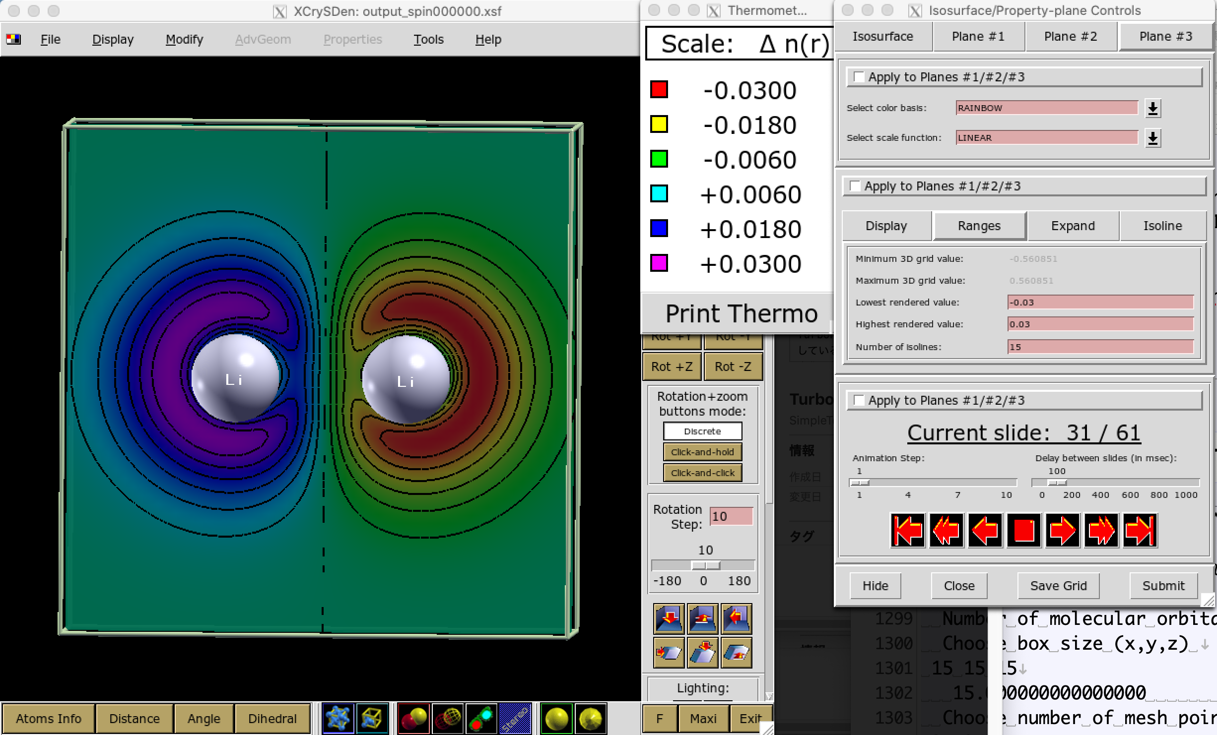
Thus, one can obtain an AFM trial wavefunction.
04-04 Li2 dimer and Li atom: Convert JDFT WF to JAGPu one
Next step is to convert the optimized JDFT ansatz to a JAGPu one. You should check the consistency after conversion.
Change working directory:
% cd ../../02convert_WF_JDFT_to_JAGP
copy
fort.10obtained from DFT calculation:% cp ../01trial_wavefunction/01DFT/fort.10_new ./fort.10_in
copy
makefort10.input, and edit:% cp ../01trial_wavefunction/00makefort10/makefort10.input . % sed -i -e '/&symmetries/a nosym_contr=.true.' makefort10.input % sed -i -e '/nshelljas/a ndet_hyb=2' makefort10.input
run makefort10
% makefort10.x < makefort10.input > out_make
% mv fort.10_new fort.10_out
convert wavefunction
% convertfort10-serial.x < convertfort10.input > out_conv
% mv fort.10_new fort.10
run correlated sampling for conversion check
% cd ../03conversion_check
% cp ../02convert_WF_JDFT_to_JAGP/fort.10 .
% cp ../02convert_WF_JDFT_to_JAGP/fort.10_in fort.10_corr

% turborvb-serial.x < datasvmc.input > out_vmc
% readforward-serial.x < datasvmc.input > out_read
Li2 dimer:
% cat corrsampling.dat

Number of bins                146
reference energy: E(fort.10)  -0.149056547E+02     0.903277814E-02
reweighted energy: E(fort.10_corr)  -0.149153980E+02     0.890288018E-02
reweighted difference: E(fort.10)-E(fort.10_corr)    0.974326537E-02     0.795833755E-03
Overlap square : (fort.10,fort.10_corr)    0.993230204E+00     0.284523743E-03
Li atom:
% cat corrsampling.dat

Number of bins                146
reference energy: E(fort.10)  -0.148896680E+02     0.929468673E-02
reweighted energy: E(fort.10_corr)  -0.148896681E+02     0.929468634E-02
reweighted difference: E(fort.10)-E(fort.10_corr)    0.124625377E-07     0.316227766E-07
Overlap square : (fort.10,fort.10_corr)    0.999999997E+00     0.316227766E-07
04-05 Li2 dimer and Li atom: Optimization (WF=JAGPu)
Now that you have obtained a good trial JAGPu wavefunction, you can optimize its nodal surface at the VMC level.
Change working directory:
% cd ../04optimization
Then, copy the converted WF.
% cp ../02convert_WF_JDFT_to_JAGP/fort.10 ./
% cp fort.10 fort.10_dft
Prepare datasmin.input:
&simulation
itestr4=-4
ngen=200000
iopt=1
maxtime=10800
/
&pseudo
/
&vmc
/
&optimization
nweight=2000
nbinr=20
iboot=0
tpar=3.5d-1
parr=5.0d-3
npbra=5
parcutpar=4.5d0
/
&readio
/
¶meters
iesd=1
iesfree=1
iessw=1
iesup=1
/
The difference from datasmin.input in 03JsAGPs/03optimization is iessw,
because we optimize the determinant part (nodal surface) at this step.
Run a VMC-opt run.
% #run vmc-opt
% turborvb-serial.x < datasmin.input > out_min

% #average fort.10
% readalles.x << ____EOS
1 81 1 0
0
1000
____EOS
The rest of the procesure (e.g., averaging the variational parameters) is the same.
Warning
For a real run (i.e., for a peer-reviewed paper), one should optimize variational parameters much more carefully. We recommend that one consult to an expert user or a developer of TurboRVB, or carefully read the Wavefunction optimization part.
04-06 Li2 dimer and Li atom: VMC and LRDMC
VMC and LRDMC procesures are the same as in the JsAGPs case.
VMC
First, create a working directory, and copy the trial wavefunction:
% cd ../05vmc/
% cp ../04optimization/fort.10 .
Then, copy
datasmin.inputand rename it asave.in:% cp ../04optimization/datasmin.input ave.in
You must also rewrite value of
ngenin ave.in asngen=1, andioptasiopt=1, by using an editor or typing the following commands:% sed -i -e 's/ngen=.*/ngen=1/g' ave.in % sed -i -e 's/iopt=.*/iopt=1/g' ave.in
Next, change
I/O flagin fort.10 to1which allow us to write the optimized variationa parameters:% sed -i -e '/unconstrained/{n;s/0$/1/}' fort.10
Note
You may need to use GNU sed
gsedinstead ofsedon macOS.Run the dummy VMC by typing
% turborvb-serial.x < ave.in > out_ave
Next step is to run VMC for calculating the total energy. Prepare
datasvmc.input, and run a VMC calculation by typing:% turborvb-serial.x < datasvmc.input > out_vmc
After the VMC run finishes, check the total energy by running the script:
% forcevmc.sh 10 2 1
A reblocked total energy and its variance is written in
pip0.d.
LRDMC
Prepare different working directories for each value of alat, copy fort.10 to each directory, and create an input file datasfn.input with the corresponding alat:
alat_0.8Z
alat_1.0Z
alat_1.2Z
alat_1.5Z
Then, run each LRDMC calculation after generating initial electron configurations at the VMC level.
cd ../06lrdmc/
cp ../05vmc/fort.10 .

lrdmc_root_dir=`pwd`

alat_list="0.8Z 1.0Z 1.2Z 1.5Z"
for alat in $alat_list
do
    cd alat_${alat}
    cp ${lrdmc_root_dir}/fort.10 ./fort.10
    turborvb-serial.x < datasvmc.input > out_vmc
    turborvb-serial.x < datasfn.input > out_fn
    cd ${lrdmc_root_dir}
done

num=0
echo -n > ${lrdmc_root_dir}/evsa.gnu
for alat in $alat_list
do
    cd alat_${alat}
    num=`expr ${num} + 1`
    echo "10 20 5 1" | readf.x
    alat_d=`grep alat= datasfn.input | cut -f 2 -d '='`
    echo -n "${alat_d} " >> ${lrdmc_root_dir}/evsa.gnu
    tail -n 1 fort.20 | awk '{print $1, $2}' >> ${lrdmc_root_dir}/evsa.gnu
    cd ${lrdmc_root_dir}
done

sed "1i 2  ${num}  4  1" evsa.gnu > evsa.in

funvsa.x < evsa.in > evsa.out
Li2 dimer
HF = -14.8715 Ha
VMC(JDFT) = -14.9759(9) Ha
LRDMC(JDFT) = -14.9894(11) Ha
VMC(JsAGPs) = -14.9821(4) Ha
LRDMC(JsAGPs) = -14.991(1) Ha
VMC(JAGPu) = -14.9819(5) Ha
LRDMC(JAGPu) = -14.990(1) Ha
Exact = -14.9951 Ha
Li atom
HF = -7.4327 Ha
VMC(JDFT) = -7.4754(3) Ha
LRDMC(JDFT) = -7.4779(5) Ha
VMC(JsAGPs) = -7.477(2) Ha
LRDMC(JsAGPs) = -7.4783(4) Ha
VMC(JAGPu) = -7.477(3) Ha
LRDMC(JAGPu) = -7.4791(4) Ha
Exact = -7.4781 Ha
Binding energy
Ebond = 38.9 mHa (experiment)
05 Li2 dimer and Li atom - JAGP (JPf) ansatz
05-01 (spin-unpolarized case) Li2 dimer: Convert JDFT WF to JAGP one
The most important procedure in a Pfaffian calculation is to convert a JDFT or JAGPu ansatz to JAGP(JPf) ansatz. Since the JAGP ansatz is a special case of the JPf one, where only \(G_{ud}\) and \(G_{du}\) terms are defined as described in the section review paper, the conversion can be realized just by direct substitution. Therefore, the main challenge is to find a reasonable initialization for the two spin-triplet sectors \(G_{uu}\) and \(G_{dd}\) that are not described in the JAGP and that otherwise have to be set to 0. There are two possible approaches to convert an ansatz: (i) for polarized systems, we can build the \(G_{uu}\) block of the matrix by using an even number of \(\{ \phi_i\}\) and build an antisymmetric \(g_{uu}\), where the eigenvalues \(\lambda_k\) are chosen to be large enough to occupy certainly these unpaired states, as in the standard Slater determinant used for our initialization. Again, we emphasize that this works only for polarized systems. (ii) The second approach that also works in a spin-unpolarized case is to determine a standard broken symmetry single determinant ansatz (e.g., by TurboRVB built-in DFT within the LSDA) and modify it with a global spin rotation. Indeed, in the presence of finite local magnetic moments, it is often convenient to rotate the spin moments of the WF in a direction perpendicular to the spin quantization axis chosen for our spin-dependent Jastrow factor, i.e., the \(z\) quantization axis. In this way one can obtain reasonable initializations for \(G_{uu}\) and \(G_{dd}\). TurboRVB allows every possible rotation, including an arbitrary small one close to the identity. A particularly important case is when a rotation of \(\pi/2\) is applied around the \(y\) direction. This operation maps \(|\uparrow \rangle \rightarrow \frac{1} {\sqrt{2}} \left( | \uparrow \rangle + |\downarrow \rangle \right) \mbox{ and } |\downarrow \rangle \rightarrow \frac 1 {\sqrt{2}} \left( | \uparrow \rangle - |\downarrow \rangle \right).\) One can convert from a AGP the pairing function that is obtained from a VMC optimization \({g_{ud}}(\mathbf{i},\mathbf{j}) = {f_S}({{\mathbf{r}}_i},{{\mathbf{r}}_j})\frac{{\left| { \uparrow \downarrow } \right\rangle - \left| { \downarrow \uparrow } \right\rangle }}{{\sqrt 2 }} + {f_T}({{\mathbf{r}}_i},{{\mathbf{r}}_j})\frac{{\left| { \uparrow \downarrow } \right\rangle + \left| { \downarrow \uparrow } \right\rangle }}{{\sqrt 2 }}\) to a Pf one \({g_{ud}}(\mathbf{i},\mathbf{j}) \to g\left( {\mathbf{i},\mathbf{j}} \right){\text{ }} = {f_S}({{\mathbf{r}}_i},{{\mathbf{r}}_j})\frac{{\left| { \uparrow \downarrow } \right\rangle - \left| { \downarrow \uparrow } \right\rangle }}{{\sqrt 2 }} + {f_T}({{\mathbf{r}}_i},{{\mathbf{r}}_j})\left( {\left| { \uparrow \uparrow } \right\rangle - \left| { \downarrow \downarrow } \right\rangle } \right).\) This transformation provides a meaningful initialization to the Pfaffian WF that can be then optimized for reaching the best possible description of the ground state within this ansatz.
The strategy (ii) is employed for the Li dimer (i.e., unpolarized case) while (i) is employed for the Li atom (i.e., polarized case)
Change working directory:
% cd ../../../05JAGP/02Li_atom/01convert_WF_JDFT_to_JAGP
First, copy
fort.10from JAGPu ansatz, and run VMC for corrlated sampling.% cp ../../../04JAGPu/01Li2_dimer/01trial_wavefunction/01DFT/fort.10_new fort.10_in % cp fort.10_in fort.10_dft % cp fort.10_dft fort.10 % turborvb-serial.x < datasvmc.input > out_vmc % rm fort.10
Convert wavefunction from JDFT ansatz to uncontracted JAGP ansatz:
% cp ../../../04JAGPu/01Li2_dimer/01trial_wavefunction/00makefort10/makefort10.input makefort10_agp_uncont.input

% makefort10.x < makefort10_agp_uncont.input > out_make_agp_uncont
% mv fort.10_new fort.10_out

% convertfort10-serial.x < convertfort10.input > out_conv_agp_uncont
% mv fort.10_new fort.10_agp_uncont
Run correlated sampling
% cp fort.10_dft fort.10
% cp fort.10_agp_uncont fort.10_corr
% readforward-serial.x < datasvmc.input > out_readforward
% mv corrsampling.dat corrsampling_dft_agp_uncont.dat
% rm fort.10
% cat corrsampling_dft_agp_uncont.dat

Number of bins                146
reference energy: E(fort.10)  -0.148896680E+02     0.929468674E-02
reweighted energy: E(fort.10_corr)  -0.148896681E+02     0.929468647E-02
reweighted difference: E(fort.10)-E(fort.10_corr)    0.122986368E-07     0.316227766E-07
Overlap square : (fort.10,fort.10_corr)    0.999999997E+00     0.316227766E-07
Convert wavefunction from uncontracted JAGP ansatz to uncontracted JPf (norotate) ansatz:
% cp fort.10_agp_uncont fort.10_in
% cp makefort10_agp_uncont.input makefort10_pf_uncont.input
Edit
makefort10_pf_uncont.input% sed -i -e '/&system/a yes_pfaff=.true.' -e '/&symetries/a rot_pfaff=.false.' makefort10_pf_uncont.input
Convert wavefunction
% makefort10.x < makefort10_pf_uncont.input > out_make_pfaff_uncont
% mv fort.10_new fort.10_out

% convertpfaff.x norotate > out_conv_pfaff_norotate

% cp fort.10_new fort.10_pfaff_uncont
Run correlated sampling
% cp fort.10_dft fort.10
% cp fort.10_pfaff_uncont fort.10_corr

% readforward-serial.x < datasvmc.input > out_readforward
% mv corrsampling.dat corrsampling_agp_pfaff_uncont.dat
% cat corrsampling_agp_pfaff_uncont.dat

Number of bins                146
reference energy: E(fort.10)  -0.148896680E+02     0.929468674E-02
reweighted energy: E(fort.10_corr)  -0.148896681E+02     0.929468647E-02
reweighted difference: E(fort.10)-E(fort.10_corr)    0.122986368E-07     0.316227766E-07
Overlap square : (fort.10,fort.10_corr)    0.999999997E+00     0.316227766E-07
Convert wavefunction from uncontracted JPf ansatz to contracted JPf ansatz:
% cp fort.10_pfaff_uncont fort.10_in
% cp makefort10_pf_uncont.input makefort10_pf_cont.input
Edit makefort10_pf_cont.input
% sed -i -e '/&symmetries/a nosym_contr=.true.' -e '/nshelljas/a ndet_hyb=2' makefort10_pf_cont.input
Convert wavefunction
% makefort10.x < makefort10_pf_cont.input > out_make_pfaff_cont
% mv fort.10_new fort.10_out

% convertfort10-serial.x < convertfort10.input > out_conv_pfaff_cont

% cp fort.10_new fort.10_pfaff_cont
% cp fort.10_pfaff_cont fort.10_corr
Run correlated sampling
% cp fort.10_dft fort.10
% readforward-serial.x < datasvmc.input > out_readforward
% mv corrsampling.dat corrsampling_dft_pfaff_cont.dat
% cat corrsampling_dft_pfaff_cont.dat

Number of bins                146
reference energy: E(fort.10)  -0.148896680E+02     0.929468674E-02
reweighted energy: E(fort.10_corr)  -0.148896681E+02     0.929468645E-02
reweighted difference: E(fort.10)-E(fort.10_corr)    0.115194734E-07     0.316227766E-07
Overlap square : (fort.10,fort.10_corr)    0.999999997E+00     0.505322962E-07
Rotate wavefunction by 1/8 pi:
% cp fort.10_pfaff_cont fort.10_in
% cp fort.10_pfaff_cont fort.10_out
% echo "-0.125" | convertpfaff.x > out_conv_pfaff_rot

% cp fort.10_new fort.10_pfaff_cont_rot
Clean fort.10
% cp fort.10_pfaff_cont_rot fort.10
% cleanfort10.x
% mv fort.10_clean fort.10

% cp fort.10 fort.10_final
% cp fort.10 fort.10_corr
Run correlated sampling
% cp fort.10_dft fort.10
% readforward-serial.x < datasvmc.input > out_readforward
% mv corrsampling.dat corrsampling_dft_pfaff_cont_rot.dat
% rm fort.10
% cat corrsampling_dft_pfaff_cont_rot.dat

Number of bins                146
reference energy: E(fort.10)  -0.148896680E+02     0.929468674E-02
reweighted energy: E(fort.10_corr)  -0.148904372E+02     0.936290264E-02
reweighted difference: E(fort.10)-E(fort.10_corr)    0.769116534E-03     0.396919093E-03
Overlap square : (fort.10,fort.10_corr)    0.998728350E+00     0.512541253E-03
The total energy was a bit lost by the rotation.
Note
If you want to use a more general spin-dependent Jastrow, i.e., independent parameters for the parallel and opposite spins (twobody = -27), you should manually put variational parameters for the two-body Jastrow part whenever generating a new fort.10.
05-02 (spin-polarized case) Li atom: Convert JDFT WF to JAGP one
Change working directory:
% cd ../../../05JAGP/02Li_atom/01convert_WF_JDFT_to_JAGP
First, copy
fort.10from JAGPu ansatz, and run VMC for correlated sampling.% cp ../../../04JAGPu/02Li_atom/01trial_wavefunction/01DFT/fort.10_new fort.10_in % cp fort.10_in fort.10_dft % cp fort.10_dft fort.10 % turborvb-serial.x < datasvmc.input > out_vmc % rm fort.10
Convert wavefunction from JDFT ansatz to uncontracted JAGP ansatz:
% cp ../../../04JAGPu/02Li_atom/01trial_wavefunction/00makefort10/makefort10.input makefort10_agp_uncont.input

% makefort10.x < makefort10_agp_uncont.input > out_make_agp_uncont
% mv fort.10_new fort.10_out

% convertfort10-serial.x < convertfort10.input > out_conv_agp_uncont
% mv fort.10_new fort.10_agp_uncont
Run correlated sampling
% cp fort.10_dft fort.10
% cp fort.10_agp_uncont fort.10_corr

% readforward-serial.x < datasvmc.input > out_readforward
% mv corrsampling.dat corrsampling_dft_agp_uncont.dat
% rm fort.10
% cat corrsampling_dft_agp_uncont.dat

Number of bins                146
reference energy: E(fort.10)  -0.148896680E+02     0.929468674E-02
reweighted energy: E(fort.10_corr)  -0.148896681E+02     0.929468647E-02
reweighted difference: E(fort.10)-E(fort.10_corr)    0.122986368E-07     0.316227766E-07
Overlap square : (fort.10,fort.10_corr)    0.999999997E+00     0.316227766E-07
Convert wavefunction from uncontracted JAGP ansatz to uncontracted JPf (norotate) ansatz:
% cp fort.10_agp_uncont fort.10_in
% cp makefort10_agp_uncont.input makefort10_pf_uncont.input
Edit makefort10_pf_uncont.input
% sed -i -e '/&system/a yes_pfaff=.true.' -e '/&symetries/a rot_pfaff=.false.' makefort10_pf_uncont.input
Convert wavefunction
% makefort10.x < makefort10_pf_uncont.input > out_make_pfaff_uncont
% mv fort.10_new fort.10_out

% echo "10000" | convertpfaff.x norotate > out_conv_pfaff_norotate

% cp fort.10_new fort.10_pfaff_uncont
Run correlated sampling
% cp fort.10_dft fort.10
% cp fort.10_pfaff_uncont fort.10_corr

% readforward-serial.x < datasvmc.input > out_readforward
% mv corrsampling.dat corrsampling_agp_pfaff_uncont.dat
% cat corrsampling_agp_pfaff_uncont.dat

Number of bins                146
reference energy: E(fort.10)  -0.148896680E+02     0.929468674E-02
reweighted energy: E(fort.10_corr)  -0.148896681E+02     0.929468647E-02
reweighted difference: E(fort.10)-E(fort.10_corr)    0.122986368E-07     0.316227766E-07
Overlap square : (fort.10,fort.10_corr)    0.999999997E+00     0.316227766E-07
Convert wavefunction from uncontracted JPf ansatz to contracted JPf ansatz:
% cp fort.10_pfaff_uncont fort.10_in
% cp makefort10_pf_uncont.input makefort10_pf_cont.input
Edit makefort10_pf_cont.input
% sed -i -e '/&symmetries/a nosym_contr=.true.' -e '/nshelljas/a ndet_hyb=2' makefort10_pf_cont.input
Convert wavefunction
% makefort10.x < makefort10_pf_cont.input > out_make_pfaff_cont
% mv fort.10_new fort.10_out

% convertfort10-serial.x < convertfort10.input > out_conv_pfaff_cont

% cp fort.10_new fort.10_pfaff_cont
Clean wavefunction
% cp fort.10_pfaff_cont fort.10
% cleanfort10.x
% mv fort.10_clean fort.10

% cp fort.10 fort.10_final
% cp fort.10 fort.10_corr
Run correlated sampling
% cp fort.10_dft fort.10
% readforward-serial.x < datasvmc.input > out_readforward
% mv corrsampling.dat corrsampling_dft_pfaff_cont.dat
% cat corrsampling_dft_pfaff_cont.dat

Number of bins                146
reference energy: E(fort.10)  -0.148896680E+02     0.929468674E-02
reweighted energy: E(fort.10_corr)  -0.148896681E+02     0.929468645E-02
reweighted difference: E(fort.10)-E(fort.10_corr)    0.115194734E-07     0.316227766E-07
Overlap square : (fort.10,fort.10_corr)    0.999999997E+00     0.505322962E-07
05-03 Li2 dimer and Li atom: VMC optimization (WF=JPf)
Change working directory
% cd ../02optimization
First, copy
fort.10andmakefort10.input.For Li2 dimer:
% cp ../01convert_WF_JDFT_to_JAGP/fort.10_pfaff_cont_rot  fort.10
% cp fort.10 fort.10_sav
% cp ../01convert_WF_JDFT_to_JAGP/makefort10_pf_cont.input .
For Li atom:
% cp ../01convert_WF_JDFT_to_JAGP/fort.10_pfaff_cont fort.10
% cp fort.10 fort.10_sav
% cp ../01convert_WF_JDFT_to_JAGP/makefort10_pf_cont.input .
Run optimization
% turborvb-serial.x < datasmin.input > out_min

% cleanfort10.x
% mv fort.10_clean fort.10
Check convergence and average
% # check convergence
% readalles.x << ____EOS
1 1 0 1
0
1000
____EOS

% # average
% readalles.x << ____EOS
1 81 1 0
0
1000
____EOS
(optional) If you find many warnings in your output during optimization, do the following stabilization and continue optimization.
3.1 Perform stabilization
% # Stabilization (especially needed for an open system, Li atom)
% cp fort.10 fort.10_in
% cp fort.10 fort.10_opt

% vi convertfort10mol.input
% # you should comment out epsdgm=-1d-14 -> !epsdgm=1d-14.
% # If this value is set negative, a generated molecular orbitals are random.
% # You can start from nmolmin=1, until nmolmin=N_el/ 2.
% # and check you do not loose much energy.

% convertfort10mol-serial.x < convertfort10mol.input > out_mol_stabilized
% cp fort.10_new fort.10
3.2. Run correlated sampling (aftre the above conversion)
% cp fort.10_in fort.10_corr

% turborvb-serial.x < datasvmc.input > out_vmc
% readforward-serial.x < datasvmc.input > out_readforward
% mv corrsampling.dat corrsampling_pfaff_stabilized.dat

% cat corrsampling_pfaff_stabilized.dat
3.3. Convert back to a geminal (JAGP)
% cp ../01convert_WF_JDFT_to_JAGP/makefort10_pf_cont.input .
% cp fort.10 fort.10_in

% set -- `grep -A1 "Parameters Jastrow two body" ./fort.10_in | tail -1`
% twobodyjas=$2
% onebodyjas=$3

% echo "twobodyjas=${twobodyjas} onebodyjas=${onebodyjas}"

% sed -i \
>     -e "/twobodypar/c\ twobodypar=${twobodyjas}" \
>     -e "/onebodypar/c\ onebodypar=${onebodyjas}" \
>     makefort10_pf_cont.input

% makefort10.x < makefort10_pf_cont.input > out_make_pfaff_cont
% mv fort.10_new fort.10_out

% convertfort10-serial.x < convertfort10.input > out_conv

% cp fort.10_new fort.10
% cleanfort10.x
% mv fort.10_clean fort.10
% cp fort.10_opt fort.10_new

% copyjas.x > out_copyjas
3.4. Run optimization again
% turborvb-serial.x < datasmin.input > out_min

% cleanfort10.x
% mv fort.10_clean fort.10
Check convergence and average
% # check convergence
% readalles.x << ____EOS
1 1 0 1
0
1000
____EOS

% # average
% readalles.x << ____EOS
1 81 1 0
0
1000
____EOS
Note
If you are using a more general spin-dependent Jastrow (i.e., twobody = -27), you should manually put Jastrow parameters after generating fort.10_out by makerfort10.x.
05-04 Li2 dimer and Li atom: VMC (WF=JPf)
Please refer to the Hydrogen tutorial for the details. Here, only needed commands are shown.
First, create a working directory, and copy the trial wavefunction:
% cd ../03vmc/
% cp ../02optimization/fort.10 ./fort.10
Then, copy
datasmin.inputand rename it asave.in:% cp ../02optimization/datasmin.input ave.in
You must also rewrite value of
ngenin ave.in asngen=1, andioptasiopt=1, by using an editor or typing the following commands:% sed -i -e 's/ngen=.*/ngen=1/g' ave.in % sed -i -e 's/iopt=.*/iopt=1/g' ave.in
Next, change
I/O flagin fort.10 to1which allow us to write the optimized variationa parameters:% sed -i -e '/unconstrained/{n;s/0$/1/}' fort.10
Note
You may need to use GNU sed
gsedinstead ofsedon macOS.Run the dummy VMC by typing
% turborvb-serial.x < ave.in > out_ave
Next step is to run VMC for calculating the total energy. Prepare
datasvmc.input, and run a VMC calculation by typing:% turborvb-serial.x < datasvmc.input > out_vmc
After the VMC run finishes, check the total energy by running the script:
% forcevmc.sh 10 2 1
A reblocked total energy and its variance is written in
pip0.d.
05-05 Li2 dimer and Li atom: LRDMC (WF=JPf)
Please refer to the Hydrogen tutorial for the details. Here, only needed commands are shown.
Prepare different working directories for each value of alat, copy fort.10 to each directory, and create an input file datasfn.input with the corresponding alat:
alat_0.8Z
alat_1.0Z
alat_1.2Z
alat_1.5Z
Then, run each LRDMC calculation after generating initial electron configurations at the VMC level.
% cd ../04lrdmc/
% cp ../03vmc/fort.10 .
lrdmc_root_dir=`pwd`

alat_list="0.8Z 1.0Z 1.2Z 1.5Z"
for alat in $alat_list
do
    cd alat_${alat}
    cp ${lrdmc_root_dir}/fort.10 ./fort.10
    turborvb-serial.x < datasvmc.input > out_vmc
    turborvb-serial.x < datasfn.input > out_fn
    cd ${lrdmc_root_dir}
done

num=0
echo -n > ${lrdmc_root_dir}/evsa.gnu
for alat in $alat_list
do
    cd alat_${alat}
    num=`expr ${num} + 1`
    echo "10 20 5 1" | readf.x
    alat_d=`grep alat= datasfn.input | cut -f 2 -d '='`
    echo -n "${alat_d} " >> ${lrdmc_root_dir}/evsa.gnu
    tail -n 1 fort.20 | awk '{print $1, $2}' >> ${lrdmc_root_dir}/evsa.gnu
    cd ${lrdmc_root_dir}
done

sed "1i 2  ${num}  4  1" evsa.gnu > evsa.in

funvsa.x < evsa.in > evsa.out
Finally we got:
Li2 dimer
HF = -14.8715 Ha
VMC(JDFT) = -14.9759(9) Ha
LRDMC(JDFT) = -14.989(1) Ha
VMC(JsAGPs) = -14.9821(4) Ha
LRDMC(JsAGPs) = -14.991(1) Ha
VMC(JAGPu) = -14.9819(5) Ha
LRDMC(JAGPu) = -14.990(1) Ha
VMC(JAGP) = -14.9831(4) Ha
LRDMC(JAGP) = -14.993(1) Ha
Exact = -14.9951 Ha
Li atom
HF = -7.4327 Ha
VMC(JDFT) = -7.4754(3) Ha
LRDMC(JDFT) = -7.4779(5) Ha
VMC(JsAGPs) = -7.477(2) Ha
LRDMC(JsAGPs) = -7.4783(4) Ha
VMC(JAGPu) = -7.477(3) Ha
LRDMC(JAGPu) = -7.4791(4) Ha
VMC(JAGP) = -7.4766(3) Ha
LRDMC(JAGP) = -7.4784(4) Ha
Exact = -7.4781 Ha
Binding energy
Ebond = 38.9 mHa (experiment)