Basic workflow

This page outlines a typical path for running TurboRVB: from building or converting a trial wave function in fort.10 format, through optional DFT-based preparation, variational optimization, and finally production VMC (or related QMC) runs. The exact order depends on your project—for example, you may skip DFT if you already have a suitable fort.10—but the diagrams below show how the pieces fit together in many tutorials.

The workflow is intentionally modular: each box in the figures corresponds to tools and input files documented elsewhere in this manual. Use the reference links at the bottom to jump to command-line details and examples.

Overview

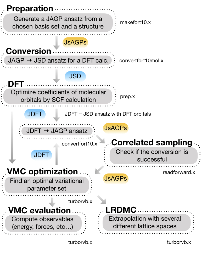
The first figure gives a high-level view: data and programs flow from an initial guess for the wave function toward optimized parameters and statistical estimates of energies and other observables.

Detailed workflow

The second figure is the detailed workflow used in the tutorial (see 01_01Hydrogen_dimer). It is more granular than the overview above and matches the step-by-step exercises you will follow there.

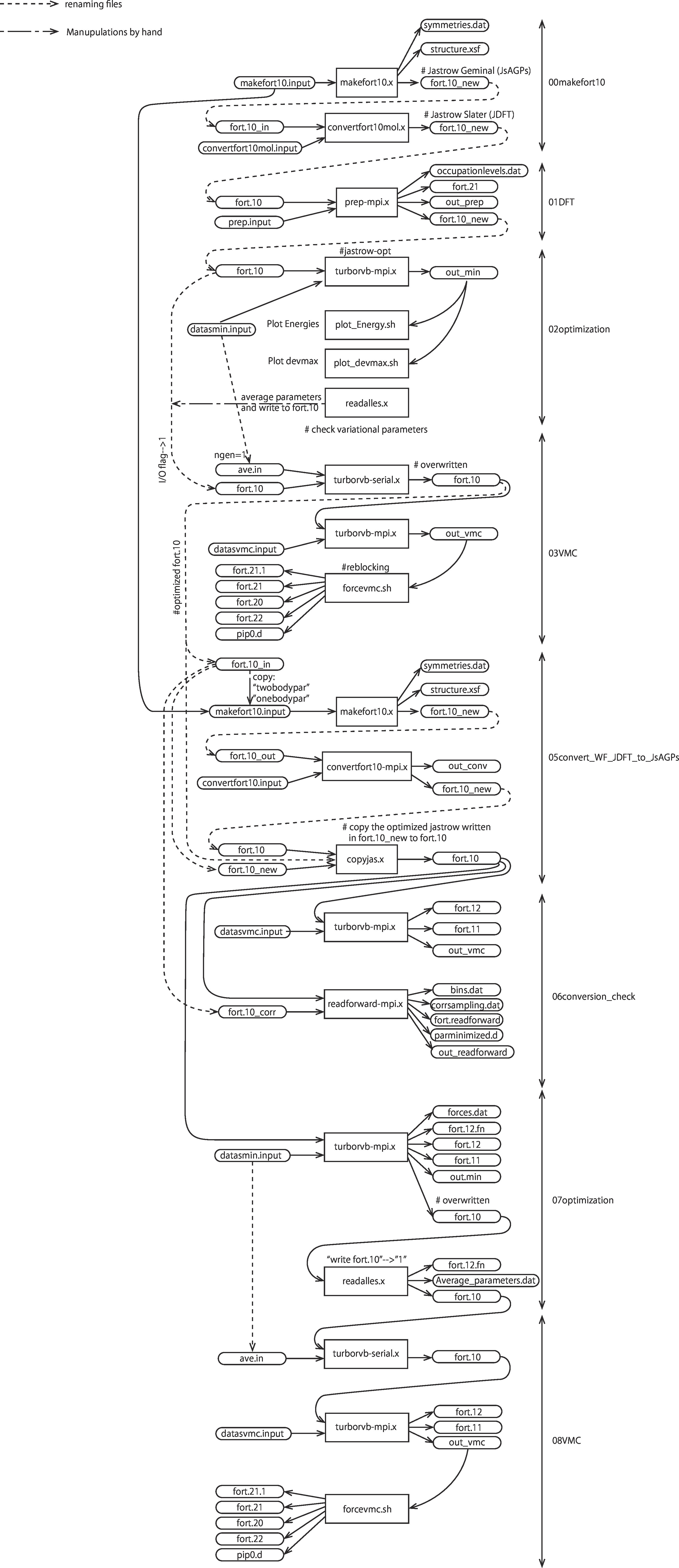
If you are working through the tutorial, treat this diagram as a roadmap: complete each stage in order unless the text explicitly says a step is optional.

Reference link

Below, each item names a stage in the workflow and points to the commands or scripts that implement it. Open the linked pages for syntax, namelists, and typical use cases.

• Prepare ``fort.10`` (trial wave function)

  You need a valid fort.10 before running turborvb.x. It can be generated from scratch, converted from another format, or adapted from a previous QMC run.

  • makefort10.x

  • convertfort10mol.x

• DFT (optional initial orbitals)

  For many molecular or solid setups, a DFT calculation (e.g. with the built-in prep machinery) provides molecular orbitals or a reasonable single-particle starting point that is then embedded or converted into TurboRVB’s Jastrow–geminal / AGP style fort.10.

  • prep.x

• Wave-function optimization

  VMC with energy minimization improves Jastrow factors, geminal/Pfaffian parameters, and possibly orbital coefficients. Monitoring tools help you judge convergence (energy, devmax, etc.) before long production runs.

  • turborvb.x

  • plot_Energy.sh, plot_NormCorr.sh, plot_devmax.sh, plot_lr.sh, plot_ratiodyn.sh

  • readalles.x

• VMC (sampling and forces)

  After optimization—or with a fixed trial wave function—you run turborvb.x for importance sampling, energies, and optionally forces. Shell helpers can post-process binary outputs.

  • turborvb.x

  • forcevmc.sh, forcevmc_kpoints.sh, forcevmc_kpoints_parallel.sh

• Convert a JDFT-style wave function to JsAGPs

  When your starting point is a JDFT (Jastrow + DFT-like) form, dedicated converters map it to a JsAGPs (Jastrow + symmetrized geminal power) representation that matches TurboRVB’s standard AGP conventions. Copy utilities can merge Jastrow and determinant pieces from different files.

  • convertfort10.x

  • copyjas.x, copydet.x

• Sanity check (conversion / forward-walking data)

  After nontrivial conversions or when using scratch output, it is good practice to verify that files are consistent and that binning or forward-walking data look reasonable before trusting long statistics.

  • readforward.x